RKToolbox Guide

Mario Berljafa, Steven Elsworth, and Stefan Güttel (The University of Manchester, UK)

Overview

Thank you for your interest in the Rational Krylov Toolbox (RKToolbox). The RKToolbox is a collection of scientific computing tools based on rational Krylov techniques. The development started in 2013 and the current version 2.9 (released in 2020) provides

an implementation of Ruhe's (block) rational Krylov sequence method [2, 5, 9, 10], allowing to control various options, including user-defined inner products, exploitation of complex-conjugate shifts, orthogonalization, rerunning [3], and simulated parallelism [4],
algorithms for the implicit and explicit relocation of the poles of a rational Krylov space [2],
a collection of utility functions and a gallery of special rational functions (e.g., Zolotarev approximants),
an implementation of RKFIT [2, 3], a robust algorithm for approximate rational least squares approximation, including automated degree reduction,
the RKFUN class [3] for numerical computations with rational functions, including support for MATLAB Variable Precision Arithmetic and the Advanpix Multiple Precision toolbox [1],
the RKFUNM class, a matrix-valued generalization of RKFUNs, together with the ability to sample and solve nonlinear eigenvalue problems using the NLEIGS [7] and AAA algorithms [8], and
the RKFUNB and BARYFUN classes [5] for numerical computations with more general rational matrix-valued formats.

This guide explains the main functionalities of the toolbox. To run the embedded MATLAB codes the RKToolbox needs to be in MATLAB's search path. For details about the installation we refer to the Download section on http://rktoolbox.org/.

Click here to view the PDF version of this guide.

Rational Krylov spaces

A (single-vector) rational Krylov space is a linear vector space of rational functions in a matrix times a vector. Let $A$ be a square matrix of size $N\times N$ , $\mathbf{b}$ an $N\times 1$ starting vector, and let $\xi_1,\xi_2,\ldots,\xi_m$ be a sequence of complex or infinite poles all distinct from the eigenvalues of $A$ . Then the rational Krylov space of order $m+1$ associated with $A,\mathbf{b},\xi_j$ is defined as

$\displaystyle \mathcal{Q}_{m+1}(A,\mathbf{b}, q_m) = q_m(A)^{-1} \mathrm{span} \{ \mathbf{b},A\mathbf{b},\ldots,A^m \mathbf{b}\},$

where $q_m(z) = \prod_{{j=1,\xi_j\neq \infty}}^m (z - \xi_j)$ is the common denominator of the rational functions associated with the rational Krylov space. The rational Krylov method by Ruhe [9, 10] computes an orthonormal basis $V_{m+1}$ of $\mathcal{Q}_{m+1}(A,\mathbf{b},q_m)$ . The basis matrix $V_{m+1}$ satisfies a rational Arnoldi decomposition of the form

$\displaystyle A V_{m+1} \underline{K_m} = V_{m+1} \underline{H_m},$

where $(\underline{H_m},\underline{K_m})$ is an (unreduced) upper Hessenberg pencil of size $(m+1)\times m$ .

Rational Arnoldi decompositions are useful for several purposes. For example, the eigenvalues of the upper $m\times m$ part of the pencil $(\underline{H_m},\underline{K_m})$ can be excellent approximations to some of $A$ 's eigenvalues [9, 10]. Other applications include matrix function approximation and rational quadrature, model order reduction, matrix equations, nonlinear eigenproblems, and rational least squares fitting (RKFIT).

Computing rational Krylov bases

Relevant functions: rat_krylov, util_cplxpair

Let us compute $V_{m+1}$ , $\underline{K_m}$ , and $\underline{H_m}$ using the rat_krylov function, and verify that the outputs satisfy the rational Arnoldi decomposition by computing the relative residual norm $\| A V_{m+1} \underline{K_m} - V_{m+1} \underline{H_m}\|_2 / \| \underline{H_m}\|_2$ . For $A$ we take the tridiag matrix of size $100$ from MATLAB's gallery, and $\mathbf{b} = [1,0,\ldots,0]^T$ . The $m=5$ poles $\xi_j$ are, in order, $-1,\infty, -\mathrm{i}, 0, \mathrm{i}$ .

N  = 100;                            % matrix size
A  = gallery('tridiag', N);
b  = eye(N, 1);                      % starting vector
xi = [-1, inf, -1i, 0, 1i];          % m = 5 poles
[V, K, H] = rat_krylov(A, b, xi);
resnorm = norm(A*V*K - V*H)/norm(H)  % residual check

resnorm =
   3.5143e-16

As some of the poles $\xi_j$ in this example are complex, the matrices $V_{m+1}$ , $\underline{K_m}$ , and $\underline{H_m}$ are complex, too:

disp([isreal(V), isreal(K), isreal(H)])

     0     0     0

However, the poles $\xi_j$ can be reordered using the function util_cplxpair so that complex-conjugate pairs appear next to each other. After reordering the poles, we can call the function rat_krylov with the 'real' option, thereby computing a real-valued rational Arnoldi decomposition [9].

% Group together poles appearing in complex-conjugate pairs.
xi = util_cplxpair(xi);
[V, K, H] = rat_krylov(A, b, xi, 'real');
resnorm = norm(A*V*K - V*H)/norm(H)
disp([isreal(V), isreal(K), isreal(H)])

resnorm =
   3.8874e-16
     1     1     1

Block rational Krylov spaces

A block Krylov space is a linear space of block vectors of size $N \times s$ built with a matrix $A$ of size ${N \times N}$ and a starting block vector $\mathbf{b} = [b_1, b_2, \ldots, b_s]$ of size ${N \times s}$ , with maximal rank. Let $\xi_1,\xi_2,\ldots,\xi_m$ be a sequence of complex or infinite poles all distinct from the eigenvalues of $A$ . Then the block rational Krylov space of order $m+1$ associated with $A,\mathbf{b},\xi_j$ is defined as

$\displaystyle \mathcal{Q}_{m+1}^{block}(A,\mathbf{b}, q_m) = q_m(A)^{-1} \left\{ \sum_{k=0}^{m} A^k \mathbf{b} C_k \right\},$

where $\{C_k\}_{k=0}^m$ are matrices of size $s \times s$ and $q_m(z) = \prod_{{j=1,\xi_j\neq \infty}}^m (z - \xi_j)$ is the common denominator of the rational matrix-valued functions associated with the block rational Krylov space. The block rational Arnoldi method [5] produces an orthonormal block matrix $\mathbf{V}_{m+1} = [\mathbf{v}_1, \ldots, \mathbf{v}_{m+1}]$ of size $N \times (m+1)s$ which satisfies a block rational Arnoldi decomposition of the form

$\displaystyle A \mathbf{V}_{m+1} \underline{\mathbf{K}_m} = \mathbf{V}_{m+1} \underline{\mathbf{H}_m},$

where $(\underline{\mathbf{H}_m},\underline{\mathbf{K}_m})$ is an (unreduced) block upper Hessenberg matrix pencil of size $(m+1)s \times ms$ . The block vectors in $\mathbf{V}_{m+1}$ blockspan the space $\mathcal{Q}_{m+1}^{block}(A,\mathbf{b},q_m)$ , that is

$\displaystyle \mathcal{Q}_{m+1}^{block}(A,\mathbf{b}, q_m) = \left\{ \sum_{k=1}^{m+1} \mathbf{v}_{k} C_k\right\},$

where the $C_k$ are arbitrary matrices of size $s \times s$ .

Block rational Krylov spaces have applications in eigenproblems with repeated eigenvalues, model order reduction, matrix equations, and for solving parameterized linear systems with multiple right-hand sides as they arise, for example, in multisource electromagnetic modelling.

Computing block rational Krylov bases

Relevant functions: rat_krylov

Let us compute $\mathbf{V}_{m+1}$ , $\underline{\mathbf{K}_m}$ , and $\underline{\mathbf{H}_m}$ using the rat_krylov function, and verify that the outputs satisfy the rational Arnoldi decomposition by computing the relative residual norm $\| A \mathbf{V}_{m+1} \underline{\mathbf{K}_m} - \mathbf{V}_{m+1} \underline{\mathbf{H}_m}\|_2 / \| \underline{\mathbf{H}_m}\|_2$ , and check the orthogonality by computing $\|\mathbf{V}_{m+1}^* \mathbf{V}_{m+1} - I \|_2$ .

N  = 100;                              % matrix size
A  = gallery('tridiag', N);
b = zeros(N, 2); b(1,1) = 1; b(7,2) = 1;
xi = [-1, inf, -1i, 0, 1i];            % m = 5 poles
[V, K, H] = rat_krylov(A, b, xi);
resnorm = norm(A*V*K - V*H)/norm(H)    % residual check
orthnorm = norm(V'*V - eye(size(V,2))) % orthogonality check

resnorm =
   4.1343e-16
orthnorm =
   6.6608e-16

The rat_krylov function also has the ability to extend the space with additional poles. When extending a block rational Krylov space, you must specify $s$ , the block size, as there is no way to infer $s$ from the existing decomposition. This is done using the parameter param.extend.

param.deflation_tol = eps(1); % default deflation tolerance
param.extend = 2;             % block size s, 1 by default
xi = 1;
[V1, K1, H1] = rat_krylov(A, V, K, H, xi, param);
resnorm = norm(A*V1*K1 - V1*H1)/norm(H1)  % residual check
orthnorm = norm(V1'*V1 - eye(size(V1,2))) % orthogonality check

resnorm =
   4.2754e-16
orthnorm =
   1.2369e-04

The loss of orthogonality occured as the columns of $\mathbf{V}_{m+1}$ become nearly linearly dependent. Removing the nearly linearly dependent vectors is called deflation. At each iteration, the block rational Arnoldi method uses an economy-size QR factorization with pivoting to detect (near) rank deficiencies. The deflation tolerance can be controlled by the parameter param.deflation_tol.

param.deflation_tol = 1e-10; % increase deflation tolerance
param.extend = 2;
xi = 1;
[V2, K2, H2, out] = rat_krylov(A, V, K, H, xi, param);
resnorm = norm(A*V2*K2 - V2*H2)/norm(H2)  % residual check
orthnorm = norm(V2'*V2 - eye(size(V2,2))) % orthogonality check

Warning: rat_krylov: 1 column deflated 
resnorm =
   6.0479e-14
orthnorm =
   6.6385e-16

Removing the linearly dependent columns from $\mathbf{V}_{m+1}$ results in an uneven block structure of the rational Arnoldi decomposition, but the orthogonality check has now passed. The residual norm has increased as the upper-Hessenberg matrix pencil still has columns containing information about the deflated vectors. Removing the corresponding columns from the pencil gives a so-called thin decomposition [5].

K2thin = K2(:,out.column_deflation);
H2thin = H2(:, out.column_deflation);
resnorm = norm(A*V2*K2thin - V2*H2thin)/norm(H2thin) % residual check

resnorm =
   4.1351e-16

Our implementation rat_krylov supports many features not shown in the basic description above.

It is possible to use matrix pencils $(A,B)$ instead of a single matrix $A$ . This leads to decompositions of the form $A \mathbf{V}_{m+1} \underline{\mathbf{K}_m} = B \mathbf{V}_{m+1} \underline{\mathbf{H}_m}$ .
Both the matrix $A$ and the pencil $(A,B)$ can be passed either explicitly, or implicitly by providing function handles to perform matrix-vector products and to solve shifted linear systems.
Non-standard inner products for constructing the orthonormal bases are supported.
One can choose between classical (CGS) and modified Gram-Schmidt orthogonalisation with or without reorthogonalization.
Iterative refinement for the linear system solves is supported.

For more details type help rat_krylov.

Moving poles of a rational Krylov space

Relevant functions: move_poles_expl, move_poles_impl

There is a direct link between the starting vector $\mathbf{b}$ and the poles $\xi_j$ of a rational Krylov space $\mathcal{Q}_{m+1}$ . A change of the poles $\xi_j$ to $\breve \xi_j$ can be interpreted as a change of the starting vector from $\mathbf{b}$ to $\mathbf{\breve b}$ , and vice versa. Algorithms for moving the poles of a rational Krylov space are described in [2] and implemented in the functions move_poles_expl and move_poles_impl.

Example: Let us move the $m=5$ poles $-1,\infty, -\mathrm{i}, 0,$ and $\mathrm{i}$ into $\breve\xi_j = -j$ , $j=1,2,\ldots,5$ .

N  = 100;
A  = gallery('tridiag', N);
b  = eye(N, 1);
xi = [-1, inf, -1i, 0, 1i];
[V, K, H] = rat_krylov(A, b, xi);
xi_new = -1:-1:-5;
[KT, HT, QT, ZT] = move_poles_expl(K, H, xi_new);

The poles of a rational Krylov space are the eigenvalues of the lower $m\times m$ part of the pencil $(\underline{\breve H_m},\underline{\breve K_m})$ in a rational Arnoldi decomposition $A \breve V_{m+1} \underline{\breve K_m} = \breve V_{m+1} \underline{\breve H_m}$ associated with that space [2]. By transforming a rational Arnoldi decomposition we are therefore effectively moving the poles:

VT = V*QT';
resnorm = norm(A*VT*KT - VT*HT)/norm(HT)
moved_poles = util_pencil_poles(KT, HT).'

resnorm =
   6.8004e-16
moved_poles =
  -1.0000e+00 + 1.1140e-16i
  -2.0000e+00 + 1.4085e-15i
  -3.0000e+00 - 7.2486e-16i
  -4.0000e+00 + 1.6407e-16i
  -5.0000e+00 - 2.4095e-16i

Rational Krylov fitting (RKFIT)

Relevant function: rkfit

RKFIT [2, 3] is an iterative Krylov-based algorithm for nonlinear rational approximation. Given two families of $N\times N$ matrices $\{F^{[j]}\}_{j=1}^{\ell}$ and $\{D^{[j]}\}_{j=1}^{\ell}$ , an $N\times n$ block of vectors $B$ , and an $N\times N$ matrix $A$ , the algorithm seeks a family of rational functions $\lbrace r^{[j]} \rbrace_{j=1}^{\ell}$ of type $(m+k, m)$ , all sharing a common denominator $q_m$ , such that the relative misfit

$\displaystyle {\rm misfit} = \sqrt{\frac{{\sum_{j=1}^\ell \| D^{[j]} [ F^{[j]}B - r^{[j]}(A)B ] \|_F^2}}{{\sum_{j=1}^\ell \| D^{[j]} F^{[j]} B \|_F^2}}}\to\min$

is minimal. The matrices $\{D^{[j]}\}_{j=1}^{\ell}$ are optional, and if not provided $D^{[j]}=I_N$ is assumed. The algorithm takes an initial guess for $q_m$ and iteratively tries to improve it by relocating the poles of a rational Krylov space.

We now show on a simple example how to use the rkfit function. Consider again the tridiagonal matrix $A$ and the vector $\mathbf{b}$ from above and let $F = A^{1/2}$ .

N  = 100;
A  = gallery('tridiag', N);
b  = eye(N, 1);
F  = sqrtm(full(A));
exact = F*b;

Now let us find a rational function $r_m(z)$ of type $(m, m)$ with $m=10$ such that $\| F \mathbf{b} - r_m(A)\mathbf{b} \|_2/\|F \mathbf{b}\|_2$ is small. The function rkfit requires an input vector of $m$ initial poles and then tries to return an improved set of poles. If we had no clue about where to place the initial poles we can easily set them all to infinity. In the following we run RKFIT for at most $15$ iterations and aim at relative misfit $\| F \mathbf{b} - r_m(A)\mathbf{b} \|_2/\|F\mathbf{b}\|_2$ below $10^{-10}$ . We display the error after each iteration.

[xi, ratfun, misfit] = rkfit(F, A, b, ...
                             repmat(inf, 1, 10), ...
                             15, 1e-10, 'real');

disp(misfit)

   7.1549e-07   1.4504e-10   4.6348e-11

The rational function $r_m(A)\mathbf{b}$ of type $(10, 10)$ approximates $A^{1/2}\mathbf{b}$ to about $10$ decimal places. A useful output of rkfit is the RKFUN object ratfun representing the rational function $r_m$ . It can be used, for example, to evaluate $r_m(z)$ :

ratfun(A,v) evaluates $r_m(A)\mathbf{v}$ as a matrix function times a vector,
ratfun(A,V) evaluates $r_m(A)V$ as a matrix function times a matrix, e.g., setting $V=I$ as the identity matrix will return the full matrix function $r_m(A)$ , or
ratfun(z) evaluates $r_m(z)$ as a scalar function in the complex plane.

Here is a plot of the error $|x^{1/2} - r_m(x)|$ over the spectral interval of $A$ (approximately $[0,4]$ ), together with the values at the eigenvalues of $A$ :

figure
ee = eig(full(A)).';
xx = sort([logspace(-4.3, 1, 500) , ee]);
loglog(xx,abs(sqrt(xx) - ratfun(xx))); hold on
loglog(ee,abs(sqrt(ee) - ratfun(ee)), 'r.', 'markers', 15)
axis([4e-4, 8, 1e-14, 1e-3]); xlabel('x'); grid on
title('| x^{1/2} - r_m(x) |','interpreter','tex')

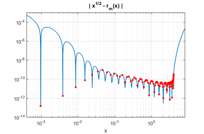
As expected the rational function $r_m(z)$ is a good approximation of the square root over $[0,4]$ . It is, however, not a uniform approximation because we are approximately minimizing the 2-norm error on the eigenvalues of $A$ , and moreover we are implicitly using a weight function given by the components of $\mathbf{b}$ in $A$ 's eigenvector basis.

Additional features of RKFIT are listed below.

An automated degree reduction procedure [3, Section 4] is implemented; it takes place if a relative misfit below tolerance is achieved, unless deactivated.
Nondiagonal rational approximants are supported; they can be specified via an additional param structure.
Adaptive incrementation of the degree controlled by a tolerance when an empty set of poles xi is provided.
Utility functions are provided for transforming scalar data appearing in complex-conjugate pairs into real-valued data, as explained in [3, Section 3.5].

For more details type help rkfit.

Some of the capabilities of RKFUN are shown in the following section.

The RKFUN class

RKFUN is the fundamental data type to represent and work with rational functions. It has already been described above how to evaluate an RKFUN object ratfun for scalar or matrix arguments by calling ratfun(z) or ratfun(A,v), respectively. There are more than 30 RKFUN methods implemented, and a list of these can be obtained by typing methods rkfun:

basis          - Orthonormal rational basis functions of an RKFUN.
coeffs         - Expansion coefficients of an RKFUN.
contfrac       - Convert an RKFUN into continued fraction form.
diff           - Differentiate an RKFUN.
disp           - Display information about an RKFUN.
double         - Convert an RKFUN into double precision (undo vpa or mp).
ezplot         - Easy-to-use function plotter for RKFUNs.
feval          - Evaluate an RKFUN at scalar or matrix arguments.
hess           - Convert an RKFUN pencil to (strict) upper-Hessenberg form.
inv            - Invert an RKFUN corresponding to a Moebius transform.
isreal         - Returns true if an RKFUN is real-valued.
minus          - Scalar subtraction.
mp             - Convert an RKFUN into Advanpix Multiple Precision format.
mrdivide       - Scalar division.
mtimes         - Scalar multiplication.
plus           - Scalar addition.
poles          - Return the poles of an RKFUN.
poly           - Convert an RKFUN into a quotient of two polynomials.
power          - Integer exponentiation of an RKFUN.
rdivide        - Division of two RKFUN.
residue        - Convert an RKFUN into partial fraction form.
rkfun          - The RKFUN constructor.
roots          - Compute the roots of an RKFUN.
size           - Returns the size of an RKFUN.
subsref        - Evaluate an RKFUN (calls feval).
times          - Multiplication of two RKFUNs.
type           - Return the type (m+k,m) of an RKFUN.
uminus         - Unary minus.
uplus          - Unary plus.
vpa            - Convert RKFUN into MATLAB's variable precision format.

The names of these methods should be self-explanatory. For example, roots(ratfun) will return the roots of ratfun, and residue(ratfun) will compute its partial fraction form. Most methods support the use of MATLAB's Variable Precision Arithmetic (VPA) and, preferably, the Advanpix Multiple Precision toolbox (MP)[1]. So, for example, contfrac(mp(ratfun)) will compute a continued fraction expansion of ratfun using multiple precision arithmetic. For more details on each of the methods, type help rkfun.<method name>.

The RKFUN gallery provides some predefined rational functions that may be useful. A list of the options can be accessed as follows:

help rkfun.gallery

  GALLERY    Collection of rational functions.
 
  obj = rkfun.gallery(funname, param1, param2, ...) takes 
  funname, a case-insensitive string that is the name of 
  a rational function family, and the family's input 
  parameters. 
 
  See the listing below for available function families.
 
  constant   Constant function of value param1.
  cheby      Chebyshev polynomial (first kind) of degree param1.
  cayley     Cayley transformation (1-z)/(1+z).
  moebius    Moebius transformation (az+b)/(cz+d) with 
             param1 = [a,b,c,d].
  sqrt       Zolotarev sqrt approximation of degree param1 on 
             the positive interval [1,param2].
  invsqrt    Zolotarev invsqrt approximation of degree param1 on 
             the positive interval [1,param2].
  sqrt0h     balanced Remez approximation to sqrt(x+(h*x/2)^2)
             of degree param3 on [param1,param2], 
             where param1 <= 0 <= param2 and h = param4.
  sqrt2h     balanced Zolotarev approximation to sqrt(x+(hx/2)^2)
             of degree param5 on [param1,param2]U[param3,param4], 
             param1 < param2 < 0 < param3 < param4, h = param6.
  invsqrt2h  balanced Zolotarev approximation to 1/sqrt(x+(hx/2)^2)
             of degree param5 on [param1,param2]U[param3,param4], 
             param1 < param2 < 0 < param3 < param4, h = param6.
  sign       Zolotarev sign approximation of degree 2*param1 on
             the union of [1,param2] and [-param2,-1].
  step       Unit step function approximation for [-1,1] of 
             degree 2*param1 with steepness param2.

Another way to create an RKFUN is to make use of MATLAB's symbolic engine. For example, r = rkfun('(x+1)*(x-2)/(x-3)^2') returns a rational function as expected. Alternatively, one can specify a rational function by its roots and poles (and an optional scaling factor) using the rkfun.nodes2rkfun function. For example, r = rkfun.nodes2rkfun([-1,2],[3,3]) will create the same rational function as above. One can also specify a rational interpolant by its barycentric representation; see the function util_bary2rkfun and reference [6].

The RKFUNM class

The RKFUNM class is the matrix-valued generalization of RKFUN. RKFUNM objects are mainly generated via the util_nleigs and util_aaa sampling routines for nonlinear eigenvalue problems. The class provides a method called linearize, which returns a matrix pencil structure corresponding to a linearization of the RKFUNM. This pencil can be used in combination with the rat_krylov function for finding eigenvalues of the linearization.

We illustrate the capabilities of the RKFUNM class with the help of a simple example. Assume we want to find numbers $z$ in the interval $[-\pi,\pi]$ where the $2\times 2$ matrix $F(z)$ defined below becomes singular:

F = @(z) [ sin(5*z) , 1 ; 1 , 1 ];

With the help of the AAA algorithm [8] we sample this matrix at sufficiently many points in the search interval and construct an accurate rational interpolant, which is then converted into RKFUNM format; see [6] for details on the conversion:

Z = linspace(-pi,pi,500);
ratm = util_aaa(F,Z)

ratm = 
	RKFUNM object of size 2-by-2 and type (21, 21).
	Real dense coefficient matrices of size 2-by-2.
	Real-valued Hessenberg pencil (H, K) of size 22-by-21.

We see that ratm is indeed an RKFUNM object representing a matrix-valued rational function of degree $21$ . In order to solve the nonlinear eigenvalue problem $F(z)v = 0$ , $v\neq 0$ , we have to linearize ratm and find the eigenvalues of the linearization near the search interval:

AB = linearize(ratm);
[A,B] = AB.get_matrices();
evs = eig(full(A), full(B));
evs = evs(abs(imag(evs))< 1e-7 & abs(evs)<pi);
figure; plot(Z,sin(5*Z));
hold on; h2 = plot(real(evs),0*evs + 1,'ro');
legend('sin(5z)','eigenvalues','Location','SouthEast')

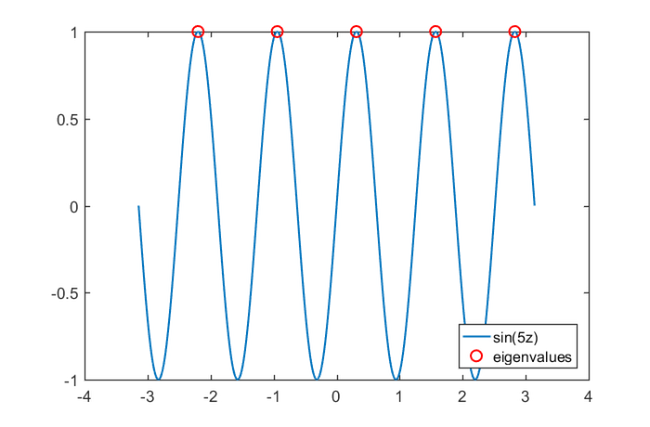
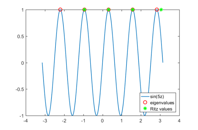
Indeed, the solutions of $\sin(5z) = 1$ are the points where $F(z)$ becomes singular. For linearizations of larger dimension the pencil AB should not be converted into matrix form using AB.get_matrices(). Instead, AB should be used as input to rat_krylov for solving the linear eigenvalue problem iteratively:

xi = zeros(1,30);             % poles of the Krylov space
[m,n] = type(ratm);
dimlin = m*size(ratm,1);      % dimension of linearization
rng(0), v = randn(dimlin, 1); % starting vector of Krylov space
[V, K, H] = rat_krylov(AB, v, xi);
ritzval = eig(H(1:end-1, :), K(1:end-1, :)); % Ritz values
ritzval = ritzval(abs(imag(ritzval))< 1e-14 & abs(ritzval)<pi);
plot(ritzval, 0*ritzval + 1, 'g*');
legend('sin(5z)','eigenvalues',...
    'Ritz values','Location','SouthEast')

The RKFUNB class

RKFUNB is a data type to represent rational matrix-valued functions of the form

$\displaystyle R_m(z) = q_m(z)^{-1}(C_0 + z C_1 + \cdots + z^m C_m),$

where $\{C_k\}_{k=0}^m$ are matrices of size $s \times s$ . The vectors computed by the block version of the rational Arnoldi method are closely linked with such functions. RKFUNBs $R_m(z)$ can be evaluated as follows:

R(A,v) evaluates $R_m(A) \circ \mathbf{v}$ as a rational matrix-valued function circed with a block vector, that is, $R_m(A) \circ \mathbf{v} = q_m(A)^{-1} ( \mathbf{v} C_0 + A \mathbf{v} C_1 + \cdots + A^m \mathbf{v} C_m),$

R(z) evaluates $R_m(z)$ at a scalar argument, giving a matrix of size $s \times s$ .

See [5] for more details.

References

[1] Advanpix LLC., Multiprecision Computing Toolbox for MATLAB, version 4.3.3.12213, Tokyo, Japan, 2017. http://www.advanpix.com/.

[2] M. Berljafa and S. Güttel. Generalized rational Krylov decompositions with an application to rational approximation, SIAM J. Matrix Anal. Appl., 36(2):894--916, 2015.

[3] M. Berljafa and S. Güttel. The RKFIT algorithm for nonlinear rational approximation, SIAM J. Sci. Comput., 39(5):A2049--A2071, 2017.

[4] M. Berljafa and S. Güttel. Parallelization of the rational Arnoldi algorithm, SIAM J. Sci. Comput., 39(5):S197--S221, 2017.

[5] S. Elsworth and S. Güttel. The block rational Arnoldi method, SIAM J. Matrix Anal. Appl., 41(2):365--388, 2020.

[6] S. Elsworth and S. Güttel. Conversions between barycentric, RKFUN, and Newton representations of rational interpolants, Linear Algebra Appl., 576:246--257, 2019.

[7] S. Güttel, R. Van Beeumen, K. Meerbergen, and W. Michiels. NLEIGS: A class of fully rational Krylov methods for nonlinear eigenvalue problems, SIAM J. Sci. Comput., 36(6):A2842--A2864, 2014.

[8] Y. Nakatsukasa, O. Sète, and L. N. Trefethen. The AAA algorithm for rational approximation, SIAM J. Sci. Comput., 40(3):A1494--A1522, 2018.

[9] A. Ruhe. Rational Krylov: A practical algorithm for large sparse nonsymmetric matrix pencils, SIAM J. Sci. Comput., 19(5):1535--1551, 1998.

[10] A. Ruhe. The rational Krylov algorithm for nonsymmetric eigenvalue problems. III: Complex shifts for real matrices, BIT, 34:165--176, 1994.