Solving large sparse eigenvalue problems
Mario Berljafa and Stefan GüttelDownload PDF or m-file
Contents
Introduction
The first use of rational Krylov methods was for the solution of large sparse eigenvalue problems  , where
  and
and  are
are  matrices and
  are the wanted eigenpairs; see [3, 4, 5, 6]. Let
  be an
be an  vector and
  a positive integer. The rational Krylov space
  is defined as
  Here,
Here,  is a polynomial of degree at most having roots
  , called poles of the rational Krylov space. If is a constant nonzero polynomial, then is a standard (polynomial) Krylov space.
The rational Arnoldi method [4, 5] can be used to compute an orthonormal basis  of
of  such that a rational Arnoldi decomposition
 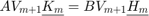 is satisfied, where
  and
and  are upper Hessenberg matrices of size
  .
.
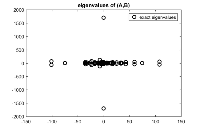
In the following we initialize two matrices for the pencil  and plot the full spectrum
  . For simplicity we take
  and choose a rather small size to be able to compute all eigenvalues exactly.
load west0479
A = west0479;
B = speye(479);
ee = eig(full(A), full(B)); % Cannot do this for larger matrices!
figure, plot(ee, 'ko', 'linewidth', 2), hold on
title('eigenvalues of (A,B)')
legend('exact eigenvalues')
We now construct a rational Krylov space with  poles all set to zero, i.e., we are interested in the generalized eigenvalues of
  closest to zero. The inner product for the rational Krylov space can be defined by the user, or otherwise is the standard Euclidean one. (Since in this example, the two coincide.)
rng(0);
b  = randn(479,1);
m  = 10;
xi = repmat(0, 1, m);
param.inner_product = @(x,y) y'*B*x;
[V, K, H] = rat_krylov(A, B, b, xi, param);

warning off, nrmA = normest(A); nrmB = normest(B); warning on
We can easily check the validity of the rational Arnoldi decomposition by veryfing that the residual norm is close to machine precision:
disp(norm(A*V*K - B*V*H)/(nrmA + nrmB))
2.6796e-18
The basis is close to orthonormal too:
disp(norm(param.inner_product(V, V)-eye(m+1)))
7.5209e-16
Extracting approximate eigenpairs
A common approach for extracting approximate eigenpairs from a search space is by using Ritz approximations or variants thereof. Let  be an matrix, and
  an
an  matrix. The pair
  is called a
- Ritz pair for with respect to
 if
if 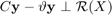 ;
; - harmonic Ritz pair for with respect to if
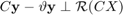 .
.
Assume that is nonsingular. It follows easily (see [1, Lemma 2.4] and [2, Theorem 2.1]) from and the definition of (harmonic) Ritz pairs given above that
- Ritz pairs
 for
for  with respect to
  arise from solutions of the generalized eigenvalue problem
  . Since
  is of full rank,
  is nonsingular, and we can equivalently solve the standard eigenvalue problem
  ;
; - harmonic Ritz pairs for with respect to arise from solutions of the generalized eigenvalue problem
 . Since
  is of full rank,
  is nonsingular, and we can equivalently solve the standard eigenvalue problem
  , and take
  .
.
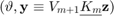
[Xr, Dr] = eig(K\H);
[Xh, Dh] = eig(H\K);
ritz = diag(Dr);
hrm_ritz = 1./diag(Dh);

plot(real(ritz), imag(ritz),'bx', 'linewidth', 3)
plot(real(hrm_ritz), imag(hrm_ritz),'m+', 'linewidth', 2)
axis([-0.02, 0.02, -0.1, 0.1])
legend('exact eigenvalues', ...
       'Ritz approximations', ...
       'harmonic Ritz')
Accuracy of the approximate eigenpairs
We can evaluate the accuracy of the (harmonic) Ritz pairs from the relative residual norm  . From the rational Arnoldi decomposition we have
  . Hence, a cheap estimate of the accuracy of an approximate eigenpair is the norm
 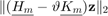 . If this norm is small compared to
  , we have computed an eigenpair of a nearby problem. It seems that in this example two eigenpairs have already converged to very high accuracy:
approx_residue = @(X) arrayfun(@(i)norm(X(:, i)), 1:size(X, 2));

approx_res = [approx_residue(H*Xr-K*Xr*Dr).' ...
              approx_residue(H*Xh-K*Xh*diag(hrm_ritz)).'];
disp(approx_res)
   5.1976e-08   4.5063e-19
   5.1976e-08   6.1961e-17
   4.5828e-08   8.2255e-07
   4.5828e-08   8.2255e-07
   6.6227e-08   1.5529e-07
   6.6227e-08   1.5529e-07
   6.6756e-08   1.5303e-07
   6.6756e-08   1.5303e-07
   1.2580e-17   2.3565e-07
   1.5728e-15   2.3565e-07
Expanding the rational Arnoldi decomposition
Let us perform  further iterations with rat_krylov, with
  repeated poles being the harmonic Ritz eigenvalues expected to converge next. Since the poles appear in complex-conjugate pairs, we can turn on the real flag for rat_krylov and end up with a real-valued quasi rational Arnoldi decomposition [6].
[~, ind] = sort(approx_res(:, 2));
xi = repmat(hrm_ritz(ind([3, 4]))', 1, 4);
param.real = 1;

[V, K, H] = rat_krylov(A, B, V, K, H, xi, param);
Let us check the residual norm of the extended rational Arnoldi decomposition, and verify that the decomposition has the original  poles at zero, and the newly selected poles.
disp(norm(A*V*K - B*V*H)/(nrmA + nrmB))
disp(util_pencil_poles(K, H).')
   2.9720e-18
   0.0000e+00 + 0.0000e+00i
   0.0000e+00 + 0.0000e+00i
   0.0000e+00 + 0.0000e+00i
   0.0000e+00 + 0.0000e+00i
   0.0000e+00 + 0.0000e+00i
   0.0000e+00 + 0.0000e+00i
   0.0000e+00 + 0.0000e+00i
   0.0000e+00 + 0.0000e+00i
   0.0000e+00 + 0.0000e+00i
   0.0000e+00 + 0.0000e+00i
   2.8261e-04 - 1.2537e-02i
   2.8261e-04 + 1.2537e-02i
   2.8261e-04 - 1.2537e-02i
   2.8261e-04 + 1.2537e-02i
   2.8261e-04 - 1.2537e-02i
   2.8261e-04 + 1.2537e-02i
   2.8261e-04 - 1.2537e-02i
   2.8261e-04 + 1.2537e-02i
Finally, the (improved)  Ritz pairs are evaluated, both standard and harmonic.
[Xr, Dr] = eig(K\H);
[Xh, Dh] = eig(H\K);

ritz = diag(Dr);
hrm_ritz = 1./diag(Dh);

approx_res = [approx_residue(H*Xr-K*Xr*Dr).' ...
              approx_residue(H*Xh-K*Xh*diag(hrm_ritz)).'];

disp(approx_res)
   7.8102e-10   8.8386e-20
   7.8102e-10   2.5844e-19
   1.0521e-09   1.2433e-13
   1.5917e-08   1.2433e-13
   3.4226e-10   3.3683e-11
   3.4226e-10   2.3079e-10
   5.3472e-10   3.5878e-13
   5.3472e-10   3.5878e-13
   1.1481e-09   2.3904e-11
   1.1481e-09   2.3904e-11
   3.9385e-09   9.2915e-09
   3.9385e-09   9.2915e-09
   6.0424e-16   4.0670e-09
   2.5439e-11   4.0670e-09
   2.5439e-11   3.3345e-09
   9.7244e-12   3.3345e-09
   9.7244e-12   9.9538e-09
   4.4158e-16   9.9538e-09
figure, plot(ee, 'ko', 'linewidth', 2), hold on
plot(real(ritz), imag(ritz),'bx', 'linewidth', 3)
plot(real(hrm_ritz), imag(hrm_ritz),'m+', 'linewidth', 2)
axis([-0.08, 0.08, -0.1, 0.1])
legend('exact eigenvalues', ...
       'Ritz approximations', ...
       'harmonic Ritz')
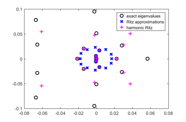
Harmonic Ritz pairs are typically better than (standard) Ritz pairs for interior eigenvalues, thought this is not yet fully understood. Also, for symmetric matrices the two sets of Ritz values interlace each other, and hence their distance is not large as ultimately both sets converge to the same eigenvalues.
References
[1] G. De Samblanx and A. Bultheel. Using implicitly filtered RKS for generalised eigenvalue problems, J. Comput. Appl. Math., 107(2):195--218, 1999.
[2] R. B. Lehoucq and K. Meerbergen. Using generalized Cayley transformations within an inexact rational Krylov sequence method, SIAM J. Matrix Anal. Appl., 20(1):131--148, 1998.
[3] A. Ruhe. Rational Krylov sequence methods for eigenvalue computation, Linear Algebra Appl., 58:391--405, 1984.
[4] A. Ruhe. Rational Krylov algorithms for nonsymmetric eigenvalue problems, Recent Advances in Iterative Methods. Springer New York, pp. 149--164, 1994.
[5] A. Ruhe. Rational Krylov: A practical algorithm for large sparse nonsymmetric matrix pencils, SIAM J. Sci. Comput., 19(5):1535--1551, 1998.
[6] A. Ruhe. The rational Krylov algorithm for nonsymmetric eigenvalue problems. III: Complex shifts for real matrices, BIT, 34(1):165--176, 1994.