The FEAST algorithm for Hermitian eigenproblems
Mario Berljafa and Stefan GüttelDownload PDF or m-file
Contents
Introduction
FEAST is an algorithm for computing a few eigenpairs  of a large sparse eigenvalue problem
  , where
  is a Hermitian
  matrix, and
  is Hermitian positive definite [4]. FEAST belongs to the class of contour-based eigensolvers which have recently attracted a lot of attention [3].
Mathematically, FEAST can be interpreted as a subspace iteration applied to a rational matrix function which serves the purpose of separating the wanted eigenvalues from the unwanted (i.e., it acts as a filter function). The RKFUN calculus of the RKToolbox is a convenient tool for working with rational functions and it allows for a simple implementation of the basic FEAST iteration. Of course, the full FEAST implementation comes with many more "bells and whistles," and in this tutorial we only aim to demonstrate the basic idea.
Model eigenvalue problem
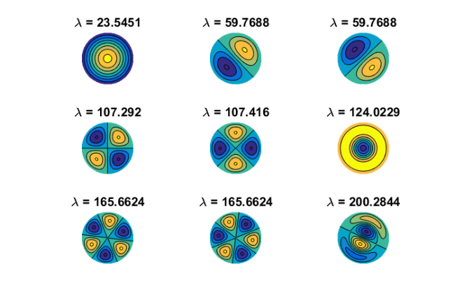
Let us consider an eigenvalue problem  , where is a finite-difference discretization of the Laplacian on a disk with homogeneous Dirichlet boundary conditions. Using MATLAB's eigs function, we first compute and visualize the
  eigenvectors corresponding to the smallest eigenvalues of :
n = 150;
G = numgrid('D', n);
A = (n+1)^2*delsq(G);
N = size(A, 1);
B = speye(N);
[V, D]   = eigs(A, 9, 'SM');
[D, ind] = sort(diag(D)); V = V(:, ind);
figure(1)
for j = 1:9
  subplot(3, 3, j)
  v = V(:, j);
  U = NaN*G;
  U(G>0) = full(v(G(G>0)));
  contourf(U);
  prism, axis square ij, axis off
  title(['\lambda = ' num2str(D(j))]);
end
Constructing the filter function
Suppose we want to find these eigenmodes using FEAST, then we need to contruct a rational filter which would separate the corresponding eigenvalues of from the others. To this end, we combine a type  step function approximation for the interval
 ![$[-1,1]$](example_feast_eq01893875229900969577.png) with a linear transformation
with a linear transformation  mapping
 ![$[0,220]$](example_feast_eq15129795111818407232.png) to
to ![$[-1,1].$](example_feast_eq03030091630708792031.png) The result is a near-optimal rational filter
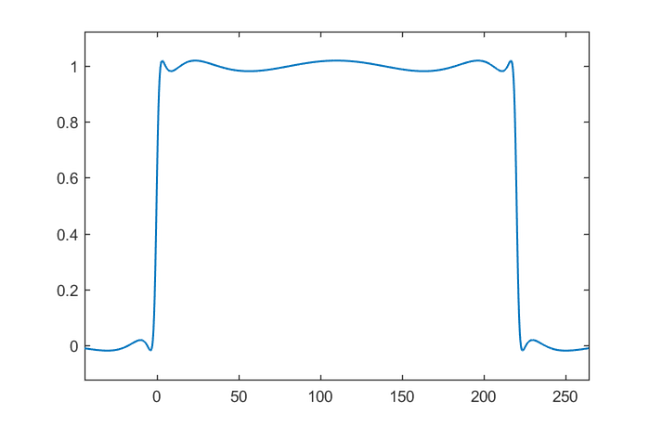
The result is a near-optimal rational filter  for the interval , attaining values very close to
  on that interval, and oscillating about
  outside:
lmin = 0; lmax = 220;
x = rkfun();                                   % independent variable x
t = 2/(lmax-lmin)*x - (lmin+lmax)/(lmax-lmin); % map [lmin,lmax] -> [-1,1]
s = rkfun('step', 5);
r = s(t);
figure, ezplot(r), hold on
Let's compute the separation ratio between the approximate values for and by finding the real local extrema of , and then finding the smallest/largest modulus of inside/outside at these extrema. Such computations can become quite sensitive, in particular with rational functions of high degree. We therefore recommend performing this using the Advanpix Multipleprecision Toolbox [1]:
r = mp(r);
extrema = roots(diff(r), 'real');
values  = r(extrema);
plot(extrema, values, 'ro')
mini = min(abs(r(extrema(lmin < extrema & extrema < lmax))));
maxi = max(abs(r(extrema(lmin > extrema | extrema > lmax))));
plot([lmin, lmax], [mini, mini], 'k--')
plot([-1e6, lmin], [maxi, maxi], 'k--')
plot([lmax,  1e6], [maxi, maxi], 'k--')
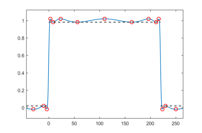
According to [2], the approximate convergence factor of FEAST for finding the eigenpairs in the interior of is given by the following ratio:
ratio = double(maxi/mini)
ratio =
   1.9351e-02
A simple FEAST implementation
We can easily verify this numerically by implementing a simple subspace iteration applied to  . Conveniently, the RKToolbox allows us to simply type
  for computing
  , the action of the rational filter on a basis
  for the search space.
% Change to double precision.
r = double(r);
% Search space basis V of dimension m.
m = 10;
V = randn(N, m);

for iter = 1:8
  % Apply rational filter to V.
  V = r(A, V);
  % Compute and sort Ritz pairs.
  Am = V'*A*V; Bm = V'*B*V;
  [W, D]   = eig(Am, Bm);
  [D, ind] = sort(diag(D)); W = W(:, ind);
  % B-normalize W.
  nrm = sqrt(diag(W'*Bm*W)); W = W/diag(nrm);
  % Form approximate eigenvectors.
  V = V*W;
  % Check residuals and number of eigenpairs inside
  % search iterval.
  Di = diag(D(lmin < D & D < lmax));
  Vi = V(:, lmin < D & D < lmax);
  resid(iter) = norm(A*Vi - B*Vi*Di, 'fro');
  nrvec(iter) = size(Vi, 2);
end
Here is a plot of the residual norms after each FEAST iteration, together with the expected convergence factor, and the number of Ritz values inside the search iterval:
figure
semilogy(resid, 'b-o'), hold on
semilogy(1e10*ratio.^(1:iter), 'k--')
for j = 1:iter
  hdl = text(j-.1,5*resid(j), num2str(nrvec(j)));
  set(hdl, 'FontSize', 14, 'Color', 'b')
end
xlim([.5, iter+.5]), xlabel('iteration')
legend('residual norm','expected rate')
ylim([1e-8, 1e6])
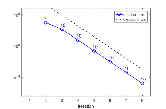
There is a very good agreement between the predicted and observed convergence. In the first iteration, no Ritz value is in the search interval, but after only  iterations we have found
  Ritz values. Indeed, looking at the 9th eigenvector in the plot above, we expect by symmetry that there will be a 10th eigenvalue corresponding to the same eigenvalue
  .
.
Remarks on parallel implementation
As mentioned above, our basic FEAST implementation is not at all efficient and serves only the purpose of a demonstration. A main feature of FEAST is its parallelism in evaluating by using a partial fraction expansion of of the form
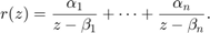
We can easily compute such an expansion using the residue command of the RKToolbox, again in multiple precision to avoid accuracy loss. Here is a plot of the poles of in the complex plane, relative to the search interval :
[alpha,beta] = residue(mp(r));
figure
plot(beta, 'ro'), hold on
plot([lmin, lmax], [0, 0], 'k-')
That's it. The following command creates a thumbnail
figure(1), hold on, plot(NaN)

References
[1] Advanpix LLC., Multiprecision Computing Toolbox for MATLAB, ver 4.3.3.12213, Tokyo, Japan, 2017. http://www.advanpix.com/.
[2] S. Güttel, E. Polizzi, P. Tang, and G. Viaud. Zolotarev quadrature rules and load balancing for the FEAST eigensolver, SIAM J. Sci. Comput., 37(4):A2100--A2122, 2015.
[3] A. Imakura, L. Du, and T. Sakurai. A map of contour integral-based eigensolvers for solving generalized eigenvalue problems, http://arxiv.org/abs/1510.02572, 2015
[4] E. Polizzi. Density-matrix-based algorithm for solving eigenvalue problems, Phys. Rev. B, 79:115112, 2009.