Pole optimization for exponential integration
Mario Berljafa and Stefan GüttelDownload PDF or m-file
Contents
Introduction
This example is concered with the computation of a family of common-denominator rational approximants for the two-parameter function  using RKFIT [2, 3]. This corresponds to the example from [3, Section 6.2]. Let us consider the problem of solving a linear constant-coefficient initial-value problem

at several time points  . The exact solutions
  are given in terms of the matrix exponential as
 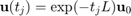 . A popular approach for approximating is to use rational functions
 ![$r^{[j]}$](example_expint_eq09359609835382356245.png) of the form
of the form
![$$
\displaystyle r^{[j]}(z) = \frac{\sigma_1^{[j]}}{\xi_1 - z} + \frac{\sigma_2^{[j]}}{\xi_2 - z} + \cdots + \frac{\sigma_m^{[j]}}{\xi_m - z},
$$](example_expint_eq16033097793306144908.png)
constructed so that ![$r^{[j]}(L)\mathbf{u}_0 \approx \mathbf{u}(t_j)$](example_expint_eq11004529826013797461.png) . Note that the poles of do not depend on
. Note that the poles of do not depend on  and we have
![$$
\displaystyle r^{[j]}(L) \mathbf{u}_0 = \sum_{i=1}^m \sigma_i^{[j]} (\xi_i I - L)^{-1} \mathbf{u}_0,
$$](example_expint_eq13758183592970566436.png)
the evaluation of which amounts to the solution of  linear systems. Such common-pole approximants have great computational advantage, in particular, in combination with direct solvers (as the LU factorizations of
  can be reused for each ) and when the linear systems are assigned to parallel processors.
Surrogate approach
In order to use RKFIT for finding "good" poles  of the rational functions , we propose a surrogate approach similar to that in [4]. Let
  be a diagonal matrix whose eigenvalues are a "sufficiently dense" discretization of the positive semiaxis
  . In this example we take
  logspaced eigenvalues in the interval
 ![$[10^{-6},10^6]$](example_expint_eq10804602582680078393.png) . Further, we define
. Further, we define  logspaced time points in the interval
 ![$[10^{-1},10^1]$](example_expint_eq14138042411722844641.png) , and the matrices
, and the matrices ![$F^{[j]} = \exp(-t_j A)$](example_expint_eq00013342048098230655.png) . We also define
. We also define ![$\mathbf{b}=[1,\ldots,1]^T$](example_expint_eq15498351051732827851.png) to assign equal weight to each eigenvalue of
to assign equal weight to each eigenvalue of  .
.
N  = 500;
ee = [0 , logspace(-6, 6, N-1)];
A  = spdiags(ee(:), 0, N, N);
b  = ones(N, 1);
t  = logspace(-1, 1, 41);
for j = 1:length(t)
  F{j} = spdiags(exp(-t(j)*ee(:)), 0, N, N);
end
We then run the RKFIT algorithm for finding a family of rational functions of type  with
with  so that
 ![$\| F^{[j]}\mathbf{b} - r^{[j]}(A)\mathbf{b} \|_2$](example_expint_eq16798110857963075828.png) is minimized for all
is minimized for all  .
.
m = 12; k = -1;              % type (11, 12)
xi = inf(1,m);               % initial poles at infinity
param.k = k;                 % subdiagonal approximant
param.maxit = 6;             % at most 6 RKFIT iterations
param.tol   = 0;             % exactly 6 iterations
param.real  = 1;             % data is real-valued
[xi, ratfun, misfit, out] = rkfit(F, A, b, xi, param);
The RKFIT outputs
The first output argument of RKFIT is a vector xi collecting the poles of the rational Krylov space. The second output ratfun is a cell array each cell of which is a rkfun, a datatype representing a rational function. All rational functions in this cell array share the same denominator with roots . The next output parameter is a vector containing the computed relative misfit after each RKFIT iteration. The relative misfit is defined as (cf. eq. (1.5) in [3])
![$$
\displaystyle \mathrm{misfit} = \sqrt{\frac{{\sum_{j=1}^\ell \| F^{[j]}\mathbf{b} - r^{[j]}(A)\mathbf{b} \|_F^2}} {{\sum_{j=1}^\ell \| F^{[j]} \mathbf{b} \|_F^2}}}.
$$](example_expint_eq09917834910523976484.png)
We can easily verify that the last entry of misfit indeed corresponds to this formula:
num = 0; den = 0;
for j = 1:length(ratfun)
  num = num + norm(F{j}*b - ratfun{j}(A,b), 'fro')^2;
  den = den + norm(F{j}*b, 'fro')^2;
end
disp([misfit(end) sqrt(num/den)])
3.6468e-05 3.6468e-05
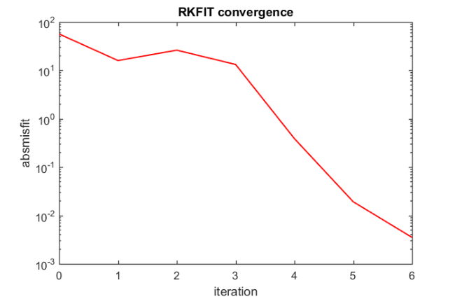
Here is a plot of the misfit vector, giving an idea of the RKFIT convergence:
figure
semilogy(0:6, [out.misfit_initial, misfit]*sqrt(den), 'r-');
xlabel('iteration');
ylabel('absmisfit')
title('RKFIT convergence')
Verifing the accuracy
To evaluate the quality of the common-denominator rational approximants for all time points , we perform an experiment similar to that in [5, Figure 6.1] by approximating and comparing the result to MATLAB's expm. Here,  is a
is a  finite-difference discretization of the scaled 2D Laplace operator
  on the domain
 ![$[-1,1]^2$](example_expint_eq04712238727479698605.png) with homogeneous Dirichlet boundary condition, and
with homogeneous Dirichlet boundary condition, and  corresponds to the discretization of
  on that domain.
% Parts of the following code have been taken from [5].
J = 30; h = 2/J; s = (-1+h:h:1-h)';  % in [3,5] J = 50 is used
[xx,yy] = meshgrid(s,s);             % 2D grid
x = xx(:); y = yy(:);                % 2D grid stretched to 1D
L = 0.02*gallery('poisson',J-1)/h^2; % 2D Laplacian
v = (1-x.^2).*(1-y.^2).*exp(x);      % initial condition
v = v/norm(v);

for j = 1:length(t)
  exac(:,j) = expm(-t(j)*L)*v;
  rat = ratfun{j}(L,v);
  err_rat(j) = norm(rat - exac(:,j));
  bnd(j) = norm(ratfun{j}(A,b) - F{j}*b,inf);
end
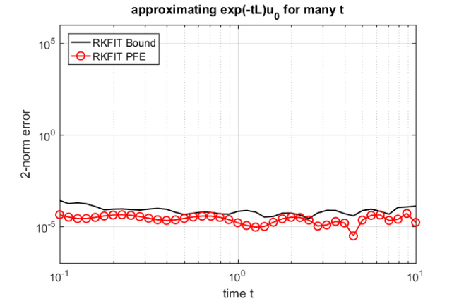
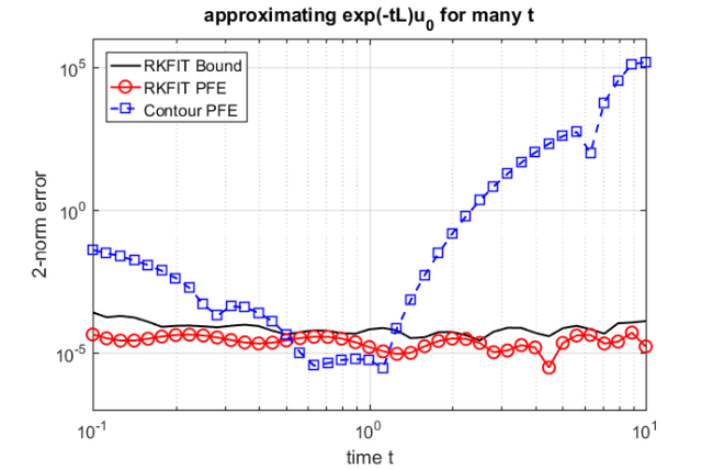
We now plot the error ![$\| \mathbf{u}(t_j) - r^{[j]}(L) \mathbf{u}_0\|_2$](example_expint_eq01585493779616005520.png) for each time point (curve with red circles), together with the approximate upper error bound
for each time point (curve with red circles), together with the approximate upper error bound ![$\| \exp(-t_j A)\mathbf{b} - r^{[j]}(A) \mathbf{b} \|_\infty$](example_expint_eq16776372825218760736.png) (black curve), which can be easily computed by direct evaluation. We find that the error is indeed approximately uniform and smaller than
(black curve), which can be easily computed by direct evaluation. We find that the error is indeed approximately uniform and smaller than  over the time interval .
figure
loglog(t, bnd, 'k-')
hold on
loglog(t, err_rat, 'r-o')
xlabel('time t'); ylabel('2-norm error')
legend('RKFIT Bound', 'RKFIT PFE', 'Location', 'NorthWest')
title('approximating exp(-tL)u_0 for many t')
grid on
axis([0.1, 10, 1e-7, 1e6])
Conversion to partial fraction form
When evaluating the rational functions on a parallel computer, it is convenient to have their partial fraction expansions at hand. The rkfun class provides a method called residue for this purpose. This method supports the use of MATLAB's variable precision (VPA) capabilities, or the Advanpix Multiple Precision (MP) toolbox [1].
For example, here are the residues and poles of the first rational function ![$r^{[1]}$](example_expint_eq01476545736979385166.png) corresponding to
corresponding to  :
:
try mp(1); catch e, try mp=@(x)vpa(x); mp(1); catch e, mp=@(x)x;
warning('MP & VPA are unavailable. Using double.'); end, end

[resid, xi, absterm, cnd, pf] = residue(mp(ratfun{1}));
disp(double([resid , xi]))
   1.1058e-01 - 4.2664e-03i  -3.9348e-01 + 1.9680e-01i
   1.1058e-01 + 4.2664e-03i  -3.9348e-01 - 1.9680e-01i
   1.2375e-01 + 9.7078e-03i  -2.7724e-01 + 6.4704e-01i
   1.2375e-01 - 9.7078e-03i  -2.7724e-01 - 6.4704e-01i
   2.7683e-01 - 2.6172e-02i  -1.3284e-01 + 1.6788e+00i
   2.7683e-01 + 2.6172e-02i  -1.3284e-01 - 1.6788e+00i
   5.0072e-01 - 4.3971e-01i   5.8293e-01 + 4.5857e+00i
   5.0072e-01 + 4.3971e-01i   5.8293e-01 - 4.5857e+00i
  -2.1039e-01 - 1.1989e+00i   4.0705e+00 + 1.1486e+01i
  -2.1039e-01 + 1.1989e+00i   4.0705e+00 - 1.1486e+01i
  -7.7942e-01 + 2.9661e-01i   1.7954e+01 + 2.5464e+01i
  -7.7942e-01 - 2.9661e-01i   1.7954e+01 - 2.5464e+01i
Comparison with contour-based approach
We now compare RKFIT with the accuracy of the contour-based rational approximants derived in [5]. As discussed there, this approach leads to approximants which are very accurate near  , but their accuracy degrades rapidly as one moves away from this parameter.
% Contour integral code from [5].
NN = 12; theta = pi*(1:2:NN-1)/NN;   % quad pts in (0, pi)
z  = NN*(.1309-.1194*theta.^2);      % quad pts on contour
z  = z + NN*.2500i*theta;
w  = NN*(-.1194*2*theta+.2500i);     % derivatives
for j = 1:length(t)
  c = (1i/NN)*exp(t(j)*z).*w;        % quadrature weights
  appr = zeros(size(v));
  for k = 1:NN/2,                    % sparse linear solves
    appr = appr - c(k)*((z(k)*speye(size(L))+L)\v);
  end
  appr = 2*real(appr);               % exploit symmetry
  err_cont(j) = norm(appr-exac(:,j));
end
loglog(t,err_cont,'b--s')
legend('RKFIT Bound', 'RKFIT PFE', 'Contour PFE', ...
       'Location', 'NorthWest')
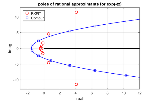
Plot of the poles
Finally, the poles of the rational functions are shown in the following plot. We can see that the "optimal" RKFIT poles do not seem to lie on a parabolic contour.
figure
hh1 = plot(xi, 'ro');
axis([-3, 12, -13, 13])
hold on

% Also plot the contour.
theta = linspace(0, 2*pi, 300);
zz = -NN*(.1309-.1194*theta.^2+.2500i*theta);
plot(zz, 'b-')
plot(conj(zz), 'b-')
hh2 = plot(-[z, conj(z)], 'bs');
plot([0, 1e3], [0, 0], 'k-', 'LineWidth', 3)
xlabel('real'), ylabel('imag')
title('poles of rational approximants for exp(-tz)')
grid on
legend([hh1, hh2], 'RKFIT', 'Contour', 'Location', 'NorthWest')
References
[1] Advanpix LLC., Multiprecision Computing Toolbox for MATLAB, ver 3.8.3.8882, Tokyo, Japan, 2015. http://www.advanpix.com/.
[2] M. Berljafa and S. Güttel. A Rational Krylov Toolbox for MATLAB, MIMS EPrint 2014.56 (http://eprints.ma.man.ac.uk/2390/), Manchester Institute for Mathematical Sciences, The University of Manchester, UK, 2014.
[3] M. Berljafa and S. Güttel. The RKFIT algorithm for nonlinear rational approximation, SIAM J. Sci. Comput., 39(5):A2049--A2071, 2017.
[4] R.-U. Börner, O. G. Ernst, and S. Güttel. Three-dimensional transient electromagnetic modeling using rational Krylov methods, Geophys. J. Int., 202(3):2025--2043, 2015. Available also as MIMS EPrint 2014.36 (http://eprints.ma.man.ac.uk/2219/).
[5] L. N. Trefethen, J. A. C. Weideman, and T. Schmelzer. Talbot quadratures and rational approximations, BIT, 46(3):653--670, 2006.