Compressing exterior Helmholtz problems

Stefan Güttel, October 2016Download PDF or m-file

Contents

Introduction

Finite difference (FD) methods are widely used for the numerical solution of partial differential equations. Due to their simplicity and potential for high computational efficiency they are often preferred to more sophisticated techniques like, e.g., finite element or spectral methods.

There is an intimite connection between FD grids, continued fractions, and rational apprpoximation, as is explained for example in [3, 4]. In particular [4] shows how to use the RKFIT method of this toolbox to 'compress' FD grids. By 'compressing an FD grid' we mean the task of computing an equivalent short-term recurrence FD grid with a small number of points that preserves essential features of the original grid. Problems like this arise, for example, when designing perfectly matched layers for the 2D variable-coefficient Helmholtz equation

$\nabla^2 u + (k_\infty^2 - c(x)) u = 0,$

for $(x,y)\in [0,+\infty)\times [0,1]$ with a compactly supported offset function $c(x)$ for the wavenumber $k_\infty$ and appropriate boundary conditions. If the transverse differential operator $-\partial_{yy}^2 - k_\infty^2$ at $x=0$ is discretized by a finite difference matrix $A$, then the above equation becomes a boundary value problem (BVP)

$\mathbf{u}''(x) = (A + c(x)I)\mathbf{u}(x),$

where the boundary conditions may be, for example, that $\mathbf{u}(0) = \mathbf{u}_0$ and $\mathbf{u}$ remains bounded for all $x\geq 0$.

It is easy to verify that the Dirichlet-to-Neumann map at $x=0$ for the above BVP is a (possibly complicated) matrix function of $A$, i.e., $\mathbf{u}'(0) = -f_h(A)\mathbf{u}_0$ (using the notation of [4]). Since its version 2.5 the RKToolbox provides a utility function util_dtnfun for the (scalar) evaluation of $f_h$, corresponding to formula (2.3) in [4].

The main aim of [4] was to approximate $f_h(A)\approx r_n(A)$ by a rational matrix function using RKFIT, and to convert the rational approximant $r_n$ into continued fraction form. This continued fration form can then be interpreted as a finite difference approximation to the original BVP, giving rise to a perfectly matched layer for variable-coefficient Helmholtz equation on unbounded domains. We refer the reader to [4] for more details. The examples below reproduce the numerical experiments in that paper.

A two-layer waveguide example

This example reproduces the two-layer waveguide example in the introduction of [4]; see in particular Figure 1.2 therein. First, let us define the transversal operator $A$, which in this case is an indefinite Helmholtz operator with wavenumber $k=k_\infty$, and the number of grid points used along the waveguide.

n = 151; k = 14;
A = (n+1)^2*gallery('tridiag',n) - k^2*speye(n);
L = 300; % length of waveguide in # grid points

Now we define the grid steps for the waveguide and replace the trailing grid steps by a Zolotarev PML [3]. (It is assumed that in the infinite layer we simply have the indefinite operator $A$ without further variation in wavenumber.)

pml = 10;                        % # of PML points
h = 1/(n+1)*ones(L+1,1); hh = h; % primal and dual grid steps
e = eig(full(A));                % spectral subintervals for Zolotarev PML
a1 = min(e(e<0)); b1 = max(e(e<0));
a2 = min(e(e>0)); b2 = max(e(e>0));
ratfun = mp(rkfun('invsqrt2h',a1,b1,a2,b2,pml,h(1)));
[hp,hd,absterm,cnd,cf] = contfrac(ratfun);
S = double([hp, hd]);

% change to PML grid
S(1,2) = S(1,2) + h(1)/2;
hx = h; hxx = hh;
hx(end+2-pml:end+1) = S(:,1);
hxx(end+1-pml:end) = S(:,2); hxx(end+1) = NaN;

Now we specify the wavenumber in the $x$ direction of the waveguide by defining the coefficient function $c(x)$, which acts as an offset for the wavenumber. The total wavenumber is $\sqrt{k_\infty^2 - c(x)}$.

c = zeros(L,1);
c(1:150) = -9^2;
c0 = c(1);
c(end-pml:end) = 0; % in the infinite PML layer we assume c = 0

We build the complete matrix system.

T = spdiags([1./([hx(2:end);NaN].*[hxx(2:end);NaN]) , ...
    -1./(hx.*hxx)-1./([hx(2:end);NaN].*hxx)-[c;NaN;NaN] , ...
    1./(hx.*[NaN;hxx(1:end-1)])],-1:1,L,L);
M = kron(T,speye(n)) - kron(speye(L),A);
u0 = zeros(n,1); u0(50) = 1/(n+1);
rhs = [ -1/(hh(2)*hh(1))*u0 ; zeros((L-1)*n,1) ];

Solve and plot.

sol = M\rhs;
Sol = [ u0, reshape(sol,n,L) ];
figure, hfig1 = pcolor(abs(Sol));
colormap pink, set(gca,'CLim',[0,7e-4])
set(hfig1,'LineStyle','none')
axis ij, title('amplitude')
hold on
plot([150,150],[0,150],'--','Color',[1,1,1])
%plot([L-pml,L-pml],[0,150],'--','Color',[1,1,1])
set(gca,'XTick',1:50:L+1,'XTickLabel',0:50:L,'YTick',1:50:n+1,'YTickLabel',0:50:n)

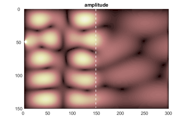
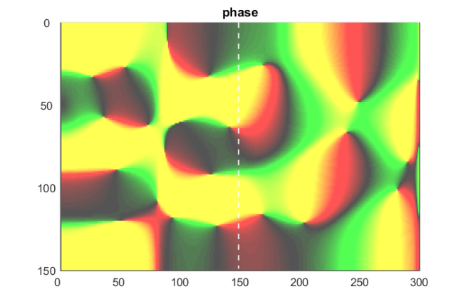
figure
Ang = angle(Sol); Ang(Ang<0) = 2*pi+Ang(Ang<0);
hfig2 = pcolor(Ang);
set(hfig2,'LineStyle','none')
axis ij, title('phase')
set(gca,'CLim',[0,2*pi])
CC = util_colormapc(1,101); CC = CC + 0.33; CC(CC>1) = 1; colormap(CC);
hold on, plot([150,150],[0,150],'--','Color',[1,1,1])
%plot([L-pml,L-pml],[0,150],'--','Color',[1,1,1])
set(gca,'XTick',1:50:L+1,'XTickLabel',0:50:L,'YTick',1:50:n+1,'YTickLabel',0:50:n)

Compute Neumann data from FD solution and compare with analytic solution:

b = hh(1)/2*(A + c0*speye(n))*u0 - (Sol(:,2)-u0)/h(1);
[U,D] = eig(full(A));
F = U*diag(util_dtnfun(h(1),[ c(end:-1:1) ; c0],diag(D)))*U';
Fu0 = U*(util_dtnfun(h(1),[ c(end:-1:1) ; c0],diag(D)).*(U'*u0));
fprintf('Number of Zolotarev-PML points for the FD problem: %d\n', pml)
fprintf('Accuracy of full FD solve w/ PML vs analytic DtN:  %e', norm(b-Fu0))

Number of Zolotarev-PML points for the FD problem: 10
Accuracy of full FD solve w/ PML vs analytic DtN:  1.351368e-04

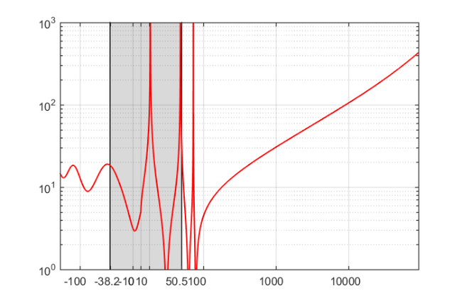
Now we plot the analytic DtN function over the spectral subintervals.

figure, hold off, semilogy(NaN), hold on
lint = util_log2lin([b1,a2],[a1,b1,a2,b2],.2);
fill([lint(1:2),lint([2,1])],[1e-25,1e-25,1e15,1e15],.85*[1,1,1],'LineStyle','-')
ax = sort([ -10.^(5:-1:1) , b1 , 0 , a2, 10.^(1:5) ]);
linax = util_log2lin(ax,[a1,b1,a2,b2],.2);
set(gca,'XTick',linax,'XTickLabel',round(10*ax)/10)
xlim([0,1]), ylim([1e-0,1e3]), grid on, set(gca,'layer','top')
xx = sort([ -logspace(log10(-a1),log10(-b1),400) , linspace(b1,a2,450) , ...
    logspace(log10(a2),log10(b2),2001), e.' , 72.89 ]);
xxt = util_log2lin(xx.',[a1,b1,a2,b2],.2).';
hh1 = semilogy(xxt,abs(util_dtnfun(h(1),[ c(end:-1:1) ; c0],xx)),'r-');

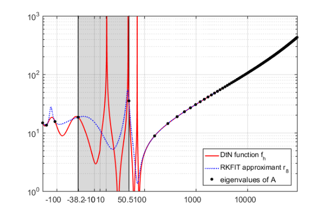
We now run RKFIT to approximate the DtN map.

param = struct;
param.k = 1;         % superdiagonal approximant
param.tol = 0;       % error tolerance
param.reduction = 0; % turn off automatic degree reduction
param.real = 0;      % no exploitation of real arithmetic
param.maxit = 30;    % maximum number of rkfit iterations
xi = inf*ones(1,7); % take m-1 initial poles
[xi,ratfun,misfit,out] = rkfit(F,A,u0,xi,param);
hh2 = semilogy(xxt,abs(ratfun(xx)),'b:');

% Plot eigenvalues on top
et = util_log2lin(e.',[a1,b1,a2,b2],.2).';
hh3 = semilogy(et,abs(util_dtnfun(h(1),[c(end:-1:1); c0],e)),'k.','MarkerSize',16);
legend([hh1,hh2,hh3],'DtN function f_h','RKFIT approximant r_8', ...
    'eigenvalues of A','Location','SouthEast');

Other examples

The other examples in [4] can be reproduced with the following scripts:

Example 6.1 - constant coefficient and 1D indefinite Laplacian

Example 6.2 - constant coefficient and 2D indefinite Laplacian

Example 6.3 - uniform approximation on indefinite interval

Example 7.1 - truly variable-coefficient case with 2D indefinite Laplacian

References

[1] Advanpix LLC., Multiprecision Computing Toolbox for MATLAB, ver 3.9.4.10481, Tokyo, Japan, 2016. http://www.advanpix.com/.

[2] M. Berljafa and S. Güttel. The RKFIT algorithm for nonlinear rational approximation, SIAM J. Sci. Comput., 39(5):A2049--A2071, 2017.

[3] V. Druskin, S. Güttel, and L. Knizhnerman. Near-optimal perfectly matched layers for indefinite Helmholtz problems, SIAM Rev., 58(1):90--116, 2016.

[4] V. Druskin, S. Güttel, and L. Knizhnerman. Compressing variable-coefficient exterior Helmholtz problems via RKFIT, MIMS EPrint 2016.53 (http://eprints.ma.man.ac.uk/2511/), Manchester Institute for Mathematical Sciences, The University of Manchester, UK, 2016.

Published with MATLAB® R2016a