Graph label propagation via RKFIT
Stefan Güttel, July 2020Download PDF or m-file
Contents
Introduction
Label propagation refers to the problem of diffusing node labels on a graph using its connectivity information. If two nodes are connected by an edge, they are considered to be more likely to share the same label. Label propagation can be used to automatically label graph nodes after only a subset of nodes has been labeled manually.
Here we consider an example from [2], where a similarity graph of images in the popular MNIST collection is constructed using a nearest neighbor search. Each image in that collection depicts a hand-written digit among  . A fraction of these images is prelabeled and the aim then is to construct ten one-against-all classifiers to recognize the other digits.
In [2], the classifiers are constructed using degree-15 polynomials of the adjacency matrix (in that paper, the degree is referred to as the number of 'taps'  ). Our aim is to demonstrate that RKFIT [1] is able to significantly compress these polynomial filters into lower-degree rational functions without sacrificing the classification performance.
Data loading
We start by loading the MNIST data set. This is available at several locations on the internet and we have used http://yann.lecun.com/exdb/mnist/, retaining the 60,000 training images with their respective labels for this experiment.
if exist('mnist.mat') ~= 2
  disp('File mnist.mat not found. Data can be downloaded from:')
  disp('http://yann.lecun.com/exdb/mnist/')
  return
end
load mnist
images = training.images;
labels = training.labels;
In order to shorten the runtime for this experiment, we will choose a small random subset of keep images, and assume that n_known of these images have known labels. The polynomial classifier is then trained on an even smaller number of n_train images.
keep = 1000;   % total number of images to work with
n_known = 150; % number of images with known labels
n_train = round(n_known/3); % training set
ind = sort(randperm(length(labels),keep));
images = images(:,:,ind); labels = labels(ind);
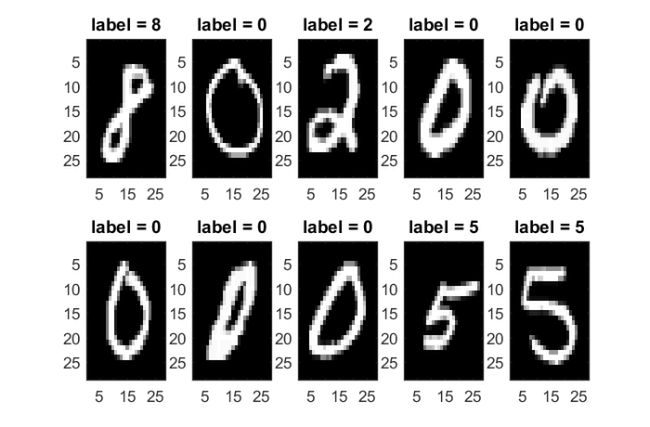
Below we visualize the first few of the selected images with their labels.
figure
for i = 1:2
    for j = 1:5
        ind = (i-1)*5+j;
        subplot(2,5,ind)
        imagesc(images(:,:,ind))
        title(['label = ' num2str(labels(ind))])
        hold on
    end
end
colormap gray; shg
Nearest neighbor adjacency
Now we construct the nearest neighbor graph having a number of keep nodes, one for each image, by connecting nodes (=images) by edges when their Frobenius norm distance is relatively small.
k = 7; AA = sparse(keep,keep);
for i = 1:keep
   Dif = repmat(images(:,:,i),1,1,keep) - images;
   for j = 1:keep
      dif(j) = norm(Dif(:,:,j),'fro');
   end
   [~,ind] = sort(dif); ind = ind(2:1+k);
   AA(i,ind) = 1;
end
A = AA' + AA; % symmetric adjacency matrix
Training the classifiers
We now follow the approach in [2] and construct, for each digit  , a polynomial classifier of degree
  . These classifiers are obtained by solving least squares problems
![$$
p^{[d]} = \mathrm{argmin}_{p\in\mathcal{P}_L} \| D^{[d]} p(A) \mathbf{t}^{[d]} - \mathbf{1} \|_2,
$$](example_digits_eq12760091143183327422.png)
where ![$D^{[d]}$](example_digits_eq02855140814159702608.png) is a diagonal matrix with diagonal entries
is a diagonal matrix with diagonal entries  (image does not depict digit
  ),
),  (image is not labeled), or
  (image depicts digit ). The vector
 ![$\mathbf t^{[d]}$](example_digits_eq10832165205875921505.png) contains
contains  to represent the labels of the training data, and
  is the vector of all ones.
The ten polynomial classifiers are used to label all images that haven't been prelabeled simply by evaluating the polynomials as ![$p^{[d]}(A)\mathbf k^{[d]}$](example_digits_eq11175882781734559794.png) , where now
, where now ![$\mathbf k^{[d]}$](example_digits_eq09611477086358278638.png) is a vector representing the known image labels. In a similar manner, we can use RKFIT to reapproximate these degree polynomials with degree-2 rational functions,
is a vector representing the known image labels. In a similar manner, we can use RKFIT to reapproximate these degree polynomials with degree-2 rational functions, ![$r^{[d]}(A)\mathbf k^{[d]} \approx p^{[d]}(A)\mathbf k^{[d]}$](example_digits_eq04447166549388138423.png) , and then use these for the labeling instead.
, and then use these for the labeling instead.
The below code implements all that and measures the classification performance of both the polynomial classifiers and the compressed RKFIT classifiers. In order to obtain measurements of some statistical robustness, we run the randomized labeling and classification several times and then average. (Note that the code is not optimized for performance and we only display its text output for the first run.)
runs = 5; % training runs for averaging of performance
Corr = []; Corr2 = []; Corrbin = []; Corrbin2 = []; Misfit = [];
for run = 1:runs
    disp(['RUN NUMBER ' num2str(run) ])
    known = sort(randperm(keep,n_known));
    train = known(sort(randperm(n_known,n_train)));
    Digit = []; Digit2 = [];
    for digit = 0:9
        lab = labels; lab(lab==digit) = -1; lab(lab~=-1) = 1;
        d = zeros(keep,1); d(known) = lab(known);
        D = spdiags(d,0,keep,keep);
        e = zeros(keep,1); e(train) = lab(train);
        E = spdiags(e,0,keep,keep);
        o = ones(keep,1);
        % construct classifier for training vector
        v = e;  % training vector
        Basis = [];
        L = 15; % degree of polynomial (taps)
        for j = 0:L
            Basis = [ Basis , D*v ];
            v = A*v; % Arnoldi procedure would be more stable!
        end
        h = pinv(Basis)*o; % get polynomial coeffs
        % apply classifier to vector of known labels
        Fd = 0*d;
        v = d; % known label vector
        M = eye(keep); F = 0*M;
        for j = 0:L
           Fd = Fd + h(j+1)*v; v = A*v;
           F = F + h(j+1)*M; M = A*M;
        end

        % degree-2 RKFIT recompression of the filter
        param = struct();
        param.deflation_tol = 0; param.real = 1;
        param.maxit = 10; param.waitbar = 0;
        param.tol = 0; param.return = 'best';
        [xi, ratfun, misfit, out] = rkfit(F, A, e, inf(1,2), param);
        Fd2 = ratfun(A,d);
        Misfit(run,digit+1) = min(misfit);

        % count number of correct binary classifications
        corrbin = sum((sign(Fd)==sign(lab)))/keep;
        Corrbin(run,digit+1) = corrbin;
        Digit = [ Digit , Fd ];
        corrbin2 = sum((sign(Fd2)==sign(lab)))/keep;
        Corrbin2(run,digit+1) = corrbin2;
        Digit2 = [ Digit2 , Fd2 ];
        if run == 1
            disp(['  Training a classifer for digit: ' num2str(digit)])
            disp(['    Correct POLY  binary classifications: ' num2str(corrbin) ])
            disp(['    Correct RKFIT binary classifications: ' num2str(corrbin2) ])
        end
    end
    % evaluate number of overall correct classifications
    [~,ind] = min(abs(Digit+1),[],2); ind = ind-1;
    corr = sum((ind==labels))/keep;
    Corr = [ Corr , corr ];
    [~,ind] = min(abs(Digit2+1),[],2); ind = ind-1;
    corr2 = sum((ind==labels))/keep;
    Corr2 = [ Corr2 , corr2 ];
    if run == 1
        disp(['  OVERALL POLY  correct classifications:  ' num2str(corr)])
        disp(['  OVERALL RKFIT correct classifications:  ' num2str(corr2)])
    else
        disp('  [output supressed]')
    end
    disp('--------------------------------------------------------------')
end
disp(['MEAN POLY  correct digit classifications: ' num2str(mean(Corr))])
disp(['MEAN RKFIT correct digit classifications: ' num2str(mean(Corr2))])
RUN NUMBER 1
  Training a classifer for digit: 0
    Correct POLY  binary classifications: 0.989
    Correct RKFIT binary classifications: 0.988
  Training a classifer for digit: 1
    Correct POLY  binary classifications: 0.973
    Correct RKFIT binary classifications: 0.976
  Training a classifer for digit: 2
    Correct POLY  binary classifications: 0.974
    Correct RKFIT binary classifications: 0.974
  Training a classifer for digit: 3
    Correct POLY  binary classifications: 0.972
    Correct RKFIT binary classifications: 0.971
  Training a classifer for digit: 4
    Correct POLY  binary classifications: 0.943
    Correct RKFIT binary classifications: 0.945
  Training a classifer for digit: 5
    Correct POLY  binary classifications: 0.936
    Correct RKFIT binary classifications: 0.929
  Training a classifer for digit: 6
    Correct POLY  binary classifications: 0.99
    Correct RKFIT binary classifications: 0.99
  Training a classifer for digit: 7
    Correct POLY  binary classifications: 0.948
    Correct RKFIT binary classifications: 0.951
  Training a classifer for digit: 8
    Correct POLY  binary classifications: 0.956
    Correct RKFIT binary classifications: 0.954
  Training a classifer for digit: 9
    Correct POLY  binary classifications: 0.922
    Correct RKFIT binary classifications: 0.944
  OVERALL POLY  correct classifications:  0.797
  OVERALL RKFIT correct classifications:  0.806
--------------------------------------------------------------
RUN NUMBER 2
  [output supressed]
--------------------------------------------------------------
RUN NUMBER 3
  [output supressed]
--------------------------------------------------------------
RUN NUMBER 4
  [output supressed]
--------------------------------------------------------------
RUN NUMBER 5
  [output supressed]
--------------------------------------------------------------
MEAN POLY  correct digit classifications: 0.775
MEAN RKFIT correct digit classifications: 0.7822
Performance evaluation
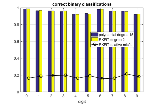
The below bar chart shows the classification accuracy for each of the ten binary (one-against-all) polynomial classifiers, and their respective RKFIT compressions. In this example we have prelabeled 150 of the 1000 images and achieved a classification accuracy above 77 %. The accuracy will increase if we prelabel a larger fraction of the images. We generally find that a degree-2 rational approximant is just as good as the degree-15 polynomial one, and in some cases even slightly better. We do not know whether this is a random artefact or if there is an explanation why the rational reapproximation can increase ("extrapolate") the classification performance. This might be of interest for future research.
figure
bar(0:9,[mean(Corrbin); mean(Corrbin2) ]')
hold on, plot((0:9)+.16,mean(Misfit),'k-o')
title('correct binary classifications')
legend('polynomial degree 15','RKFIT degree 2',...
    'RKFIT relative misfit','Location','Best')
xlim([-.5,9.5]), ylim([.0,1]), grid on, xlabel('digit');
References
[1] M. Berljafa and S. Güttel. The RKFIT algorithm for nonlinear rational approximation, SIAM J. Sci. Comput., 39(5):A2049--A2071, 2017.
[2] A. Sandryhaila and J. M. F. Moura. Discrete signal processing on graphs: Graph filters, in 2013 IEEE International Conference on Acoustics, Speech and Signal Processing, pp. 6163--6166, 2013.