Solving nonlinear eigenvalue problems
Mario Berljafa and Stefan GüttelDownload PDF or m-file
Contents
Introduction
We consider the problem of finding eigenvalues  and nonzero eigenvectors
  of a nonlinear eigenvalue problem (NLEP)

Here  is a compact target set in the complex plane and
  is a family of
  matrices depending analytically on
  . A popular approach for solving such problems is to approximate by a polynomial or rational eigenvalue problem of the form

where the  are matrices, and the
  are polynomials or rational functions in . Provided that the can be generated by a linear recursion, the problem
  can be "linearised" into a linear pencil
  of size
  , which in practice can be rather large depending on
  and
and  .
.
The NLEIGS linearisation
The NLEIGS linearisation [3] is based on rational interpolation, with the chosen as rational basis functions of the form
Here, the  are interpolation nodes on the boundary of , and the
  are poles which can be chosen freely, for example all at infinity (which leads to a polynomial interpolant) or on a singularity set
  of . The advantage of employing an interpolation-based approximation
  is that the matrices can be obtained solely by sampling
  , provided that the nodes are distinct. For more details we refer to [3, Section 2.1].
The numbers  are scaling factors which, as suggested in [3], are chosen so that
  This scaling has the advantage that the norms
  give an indication of the approximation accuracy of for ; see [3, Section 4] for more details.
Leja-Bagby sampling
To obtain a computationally efficient method it is desirable that  is a good approximation for all with a small degree parameter . This suggests to use an (asymptotically) optimal rational interpolation procedure and we propose to choose the
  as Leja-Bagby points on
  [1, 9].
More precisely, choosing  arbitrarily, we define the nodes and poles so that the following conditions are satisfied:

with the nodal functions  defined as
The Gun problem
We now demonstrate the above with an example taken from the problem collection [2]. We use the so-called gun problem, which is a model of a radio-frequency gun cavity [5]. The corresponding NLEP is
![$$ \displaystyle A(\lambda)\mathbf x = [K-\lambda M + i\sqrt{\lambda} W_1
+ i\sqrt{\lambda-108.8774^2} W_2]\mathbf x = \mathbf 0, $$](example_nlep_eq12924246813579206317.png)
where  are sparse
  matrices. Let us define a function handle to the NLEP.
if exist('nlevp') ~= 2
  disp('Function nlevp.m not found. Can be downloaded from:')
  disp(['http://www.maths.manchester.ac.uk/our-research/research-groups' ...
        '/numerical-analysis-and-scientific-computing/numerical-analysis/' ...
        'software/nlevp/'])
  return
end

[coeffs, fun] = nlevp('gun');
n = size(coeffs{1}, 1);
A = @(lam) 1*coeffs{1} - lam*coeffs{2} + ...
    1i*sqrt(lam)*coeffs{3} + ...
    1i*sqrt(lam-108.8774^2)*coeffs{4};
The target set for this problem is an upper-half disk with center  and radius
  . Note that the definition of involves two branch cuts
 ![$(-\infty,0]$](example_nlep_eq11690146182182046152.png) and
and ![$(-\infty,108.8774^2]$](example_nlep_eq16930768877730050887.png) caused by the square roots, and the union of these two is a good choice for the singularity set .
caused by the square roots, and the union of these two is a good choice for the singularity set .
We can now use the utility function util_nleigs to sample the NLEP on the target set using poles from the singularity set . The function requires as inputs a function handle to , the vertices of and represented by polygons, a tolerance for the sampling procedure, and the maximal number of terms.
Nmax  = 50;
Sigma = 62500 + 50000*exp(1i*pi*[1, linspace(0, 1)]);
Xi   = [-inf, 108.8774^2];
tol  = 1e-15;
QN   = util_nleigs(A, Sigma, Xi, tol, Nmax);
disp(QN)
	RKFUNM object of size 9956-by-9956 and type (32, 31).
	Complex sparse coefficient matrices of size 9956-by-9956.
	Complex-valued Hessenberg pencil (H, K) of size 33-by-32.
As we can see, the output of util_nleigs is an RKFUNM object QN representing , a rational matrix-valued function which interpolates at the nodes (i.e.,  for all
  ). We can evaluate
  at any point
  in the complex plane by typing QN(z). The linearize function can be used to convert into an equivalent linear matrix pencil structure
 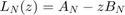 with the same eigenvalues as . Via
  we can also access the norms
  of the matrices in the expansion of . Apparently, a degree of
  was sufficient to represent to accuracy
  :
:
LN   = linearize(QN);
figure(1), semilogy(0:LN.N, LN.nrmD/LN.nrmD(1), 'r-'), grid on
legend('relative Frobenius norm of D_j'); xlabel('j')
axis([0, LN.N, 1e-16, 1])
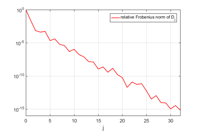
Luckily this is quite small due to the Leja-Bagby sampling strategy employed by util_nleigs. However, the full linearisation matrices are of size  and hence quite large. Here is a spy plot of .
[AN,BN] = LN.get_matrices();
figure(2)
subplot(1,2,1), spy(AN), title('A_N')
subplot(1,2,2), spy(BN), title('B_N')
The LN structure provides two function handles multiply and solve, which can be used by the rat_krylov function to compute a rational Krylov basis for without forming these matrices explicitly [7, 8]. For the rational Arnoldi algorithm we choose, rather arbitrarily,  cyclically repeated shifts in the interior of .
shifts = [9.6e+4, 7.9e+4+1.7e+4i, 6.3e+4, 4.6e+4+1.7e+4i, 2.9e+4];
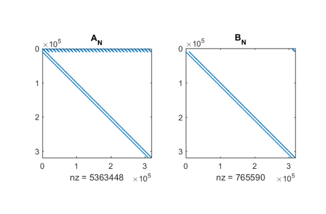
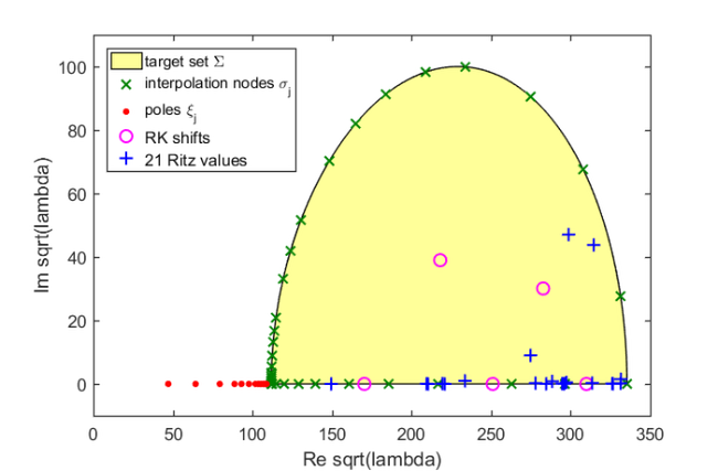
Let us first plot the target set, the sampling points , the poles , and the shifts of the rational Krylov space:
figure(3)
fill(real(sqrt(Sigma)), imag(sqrt(Sigma)), [1 1 .6])
hold on
plot(sqrt(LN.sigma), 'gx', 'Color', [0 .5 0])
plot(sqrt(LN.xi(LN.xi>0))+1i*eps, 'r.', 'MarkerSize', 14)
plot(sqrt(shifts), 'mo')
xlabel('Re sqrt(lambda)'), ylabel('Im sqrt(lambda)')
legend('target set \Sigma', 'interpolation nodes \sigma_j', ...
       'poles \xi_j', 'RK shifts', 'Location', 'NorthWest')
axis([0,350,-10,110])
The computation of the rational Arnoldi decomposition  is conveniently performed by providing the pencil structure LN as the first input argument to the rat_krylov function. Here,
  and the starting vector is chosen at random.
Note: The shifts in this example are cyclically repeated and the solve function provided in the LN structure attempts to reuse LU factors of matrices whenever possible. The five LU factors required for this example are stored automatically as persistent variables within the solve function.
v = randn(LN.N*n, 1);
shifts = repmat(shifts, 1, 14);
[V, K, H] = rat_krylov(LN, v, shifts, struct('waitbar', 1));
From the rational Arnoldi decomposition we can easily compute the Ritz pairs for the linearisation . In the following we extract the Ritz values in the interior of and find, consistently with [3], that there are 21 Ritz values. The leading elements of the corresponding Ritz vectors (normalised to unit norm) are then approximations to the eigenvectors of .
[X, D] = eig(H(1:end-1, :), K(1:end-1, :));
ritzval = diag(D);
ind = inpolygon(real(ritzval), imag(ritzval), ...
                real(Sigma), imag(Sigma));
ritzval = ritzval(ind);
ritzvec = V(1:n, 1:end)*(H*X(:, ind));
ritzvec = ritzvec/diag(sqrt(sum(abs(ritzvec).^2)));
disp(length(ritzval))
21
Let us compute the nonlinear residual norm  for all 21 Ritz pairs
  :
:
res = arrayfun(@(j) norm(A(ritzval(j))*ritzvec(:, j), 'fro'), ...
               1:length(ritzval));

figure(4)
semilogy(res, 'b-o'), xlim([1, length(res)])
legend('residual norm of Ritz pairs')
xlabel('index of Ritz pair'), hold on
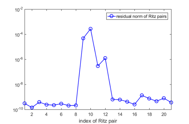
We find that all but  Ritz pairs are good approximations to the eigenpairs of the nonlinear problem. Let us run five more rational Arnoldi iterations by using as shift the mean of the four nonconverged Ritz values. This can be done by simply extending the existing rational Arnoldi decomposition.
% Use mean of Ritz values.
shifts = repmat(mean(ritzval(res>1e-8)), 1, 5);
% Extend the decomposition.
[V, K, H] = rat_krylov(LN, V, K, H, shifts, struct('waitbar',1));
Now let us compute the improved Ritz pairs and the corresponding nonlinear residuals exactly as above:
[X, D] = eig(H(1:end-1, :), K(1:end-1, :));
ritzval = diag(D);
ind = inpolygon(real(ritzval), imag(ritzval), ...
                real(Sigma),   imag(Sigma));
ritzval = ritzval(ind);
ritzvec = V(1:n, 1:end)*(H*X(:, ind));
ritzvec = ritzvec/diag(sqrt(sum(abs(ritzvec).^2)));

res = arrayfun(@(j) norm(A(ritzval(j))*ritzvec(:, j), 'fro'), ...
               1:length(ritzval));

figure(4)
semilogy(res, 'r-o')
legend('residual norm of Ritz pairs','residual norm (extended)')
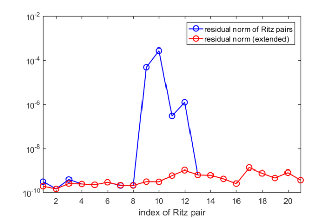
All wanted Ritz pair are now of sufficiently high accuracy and we are done. Finally, here is a plot of the Ritz values, which coincides with [3, Figure 4(a)]:
figure(3)
plot(sqrt(ritzval), 'b+')
legend('target set \Sigma', 'interpolation nodes \sigma_j', ...
       'poles \xi_j', 'RK shifts', '21 Ritz values', ...
       'Location', 'NorthWest')
Variants and extensions
The linearisation computed by util_linearise_nlep is referred to as the "static variant of NLEIGS" in [3]. The NLEIGS algorithm, which is also available online, supports the dynamic expansion of the linearisation as the rational Arnoldi iteration progresses. This dynamic expansion is inspired by the "infinite Arnoldi algorithm" presented in [4]. The CORK algorithm in [8] is a memory-efficient variant of NLEIGS which exploits the special structure of the Krylov basis vectors  associated with .
References
[1] T. Bagby. On interpolation by rational functions, Duke Math. J., 36:95--104, 1969.
[2] T. Betcke, N. J. Higham, V. Mehrmann, C. Schröder, and F. Tisseur. NLEVP: A collection of nonlinear eigenvalue problems, ACM Trans. Math. Software, 39(2):7:1--7:28, 2013.
[3] S. Güttel, R. Van Beeumen, K. Meerbergen, and W. Michiels. NLEIGS: A class of fully rational Krylov methods for nonlinear eigenvalue problems, SIAM J. Sci. Comput., 36(6):A2842--A2864, 2014.
[4] E. Jarlebring, W. Michiels, and Karl Meerbergen. A linear eigenvalue algorithm for the nonlinear eigenvalue problem, Numer. Math., 122(1):169--195, 2012.
[5] B.-S. Liao. Subspace Projection Methods for Model Order Reduction and Nonlinear Eigenvalue Computation, PhD thesis, Dept. of Mathematics, University of California at Davis, 2007.
[6] A. Ruhe. Rational Krylov algorithms for nonsymmetric eigenvalue problems, Recent Advances in Iterative Methods. Springer New York, pp. 149--164, 1994.
[7] A. Ruhe. Rational Krylov: A practical algorithm for large sparse nonsymmetric matrix pencils, SIAM J. Sci. Comput., 19(5):1535--1551, 1998.
[8] R. Van Beeumen, K. Meerbergen, W. Michiels. Compact rational Krylov methods for nonlinear eigenvalue problems, SIAM J. Matrix Anal. Appl., 36(2):820--838, 2015.
[9] J. Walsh. On interpolation and approximation by rational functions with preassigned poles, Transactions of the American Mathematical Society, 34:22--74, 1932.