Fitting an artificial frequency response

Mario Berljafa and Stefan Güttel, February 2015Download PDF or m-file

Introduction
Problem setup
Testing RKFIT
The rkfun class
Some other choices for the initial poles
Comparison with vector fitting
References

Introduction

This is an example of RKFIT being used for approximating an artifically created frequency response function $f(z)$ and finding its poles. RKFIT is described in [2, 3] and this code reproduces the example from [2, Section 5.1]. The rational function $f(z)$ is taken from [5, Section 4.1].

Problem setup

We first define a rational function $f(z)$ via its poles, residues, and the linear term. The numbers are taken from [5].

pls = [-4500,       -41000,     -100+5000i,  -100-5000i,   ...
       -120+15000i, -120-15000i,-3000+35000i,-3000-35000i, ...
       -200+45000i, -200-45000i,-1500+45000i,-1500-45000i, ...
       -500+70000i, -500-70000i,-1000+73000i,-1000-73000i, ...
       -2000+90000i,-2000-90000i];
rsd = [-3000,       -83000,      -5+7000i,   -5-7000i,     ...
       -20+18000i,  -20-18000i,   6000+45000i,6000-45000i, ...
       40+60000i,   40-60000i,    90+10000i,  90-10000i,   ...
       50000+80000i,50000-80000i, 1000+45000i,1000-45000i, ...
       -5000+92000i,-5000-92000i];

pls = pls(:);
rsd = rsd(:);
dd  = 0.2; hh = 2e-5;

f = @(zz) arrayfun(@(z) sum(rsd./(z-pls)) + dd + z*hh,zz);

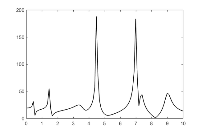
The frequency range of interest is $0$ to $100$ kHz and we can plot the response function easily. The plot should look exactly the same as [5, Figure 1], provided the number of sampling points $N$ is reduced to $100$ (in this case some peaks are missed in the plot).

figure(1)
N = 200;
zz = 1i*linspace(-1e5, 1e5, N).';
plot(abs(zz)/1e4, abs(f(zz)), 'k-')

Testing RKFIT

We now run RKFIT from [1] to compute a rational least squares approximant to $f(z)$ . To this end we need to "rewrite" the least squares problem in terms of a matrix function acting on a vector, i.e., $\| F \mathbf b - r(A)\mathbf b \|_2/\|F \mathbf b\|_2 \rightarrow \min$ . The fitting points zz will be the eigenvalues of a diagonal matrix $A$ , and $F$ will be a diagonal matrix of the fitting values. The vector $\mathbf b$ can be used for weighting the data points and we will set all weights equal to one.

A = spdiags(zz, 0, N, N);
F = spdiags(f(zz), 0, N, N);
b = ones(N, 1);

We also need to specify the initial poles of $r(z)$ . By choosing $18$ initial poles the rational function to be computed by RKFIT would be of type $(18,18)$ . However, the above rational function $f(z)$ is of type $(19,18)$ , so we need to increase the numerator degree by $k=1$ . This parameter $k$ , together with the maximal number of iterations to perform, can be given to RKFIT in form of a param structure.

init = logspace(3,5,9); % initial poles
init = [init , conj(init)];
param.k = 1;
param.maxit = 10;

That's it. Now we can run RKFIT.

[xi, ratfun, misfit_rkfit] = rkfit(F, A, b, init, param);

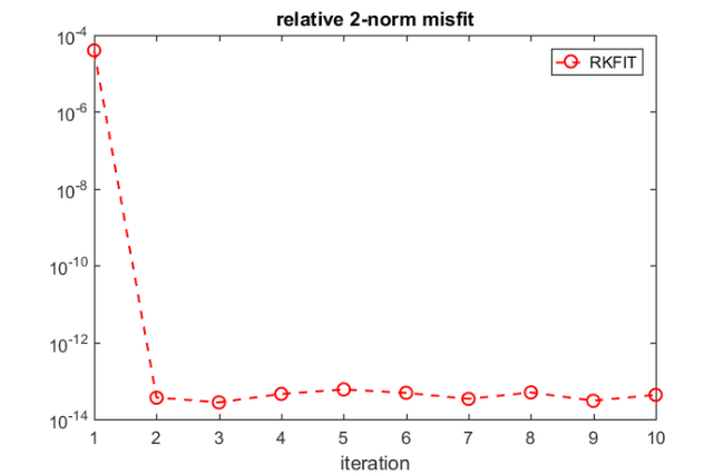
Here is a convergence plot of RKFIT, showing the relative least squares approximation error after each iteration.

figure(2)
semilogy(misfit_rkfit, 'ro--')
hold on
xlabel('iteration')
title('relative 2-norm misfit')
legend('RKFIT')

The `rkfun` class

The second output ratfun is an object of class rkfun. As expected it represents a rational function of type $(19,18)$ :

disp(ratfun)

	RKFUN object of type (19, 18).
	Complex-valued Hessenberg pencil (H, K) of size 20-by-19.
	|coeffs| = [6.236, 6.945, 6.590, 7.135, 6.829, ...]

This rational function $r(z)$ can be evaluated in two ways: The first option is to evaluate a matrix function $r(A)\mathbf b$ by calling ratfun(A,b) with two input arguments. For example, here we are calculating the relative least squares fitting error, which will coincide (up to roundoff errors) with the misfit of the last RKFIT iterate:

format shorte
disp([norm(F*b - ratfun(A, b))/norm(F*b), misfit_rkfit(end)])

   2.3020e-09   4.2950e-14

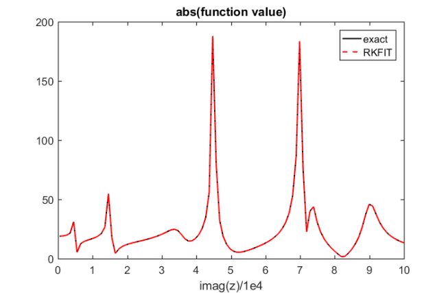
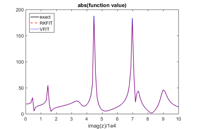
Alternatively, we can evaluate $r(z)$ pointwise by giving only one input argument. Let's compare $r(z)$ to $f(z)$ plotted before:

figure(1), hold on
plot(abs(zz)/1e4, abs(ratfun(zz)), 'r--')
xlabel('imag(z)/1e4')
title('abs(function value)')
legend('exact','RKFIT')

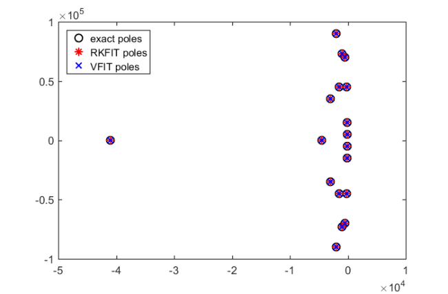
One may be interested in the poles of $r(z)$ computed by RKFIT. The poles of an rkfun can be easily retrieved using the poles method. Let us compare poles(ratfun) to the exact poles of the function $f(z)$ .

figure(3)
plot(pls,'ko'), hold on
plot(poles(ratfun),'r*')
axis([-5e4, 1e4, -1e5, 1e5])
legend('exact poles','RKFIT poles','Location','NorthWest')

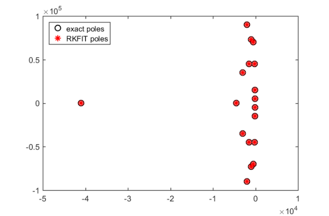
The agreement between the poles is very good.

Some other choices for the initial poles

In practice one may not know the number of poles required to fit a function to a certain accuracy. Let us see what happens if we use too many, in this case $24$ , initial poles for RKFIT.

init24 = logspace(6,9,12);
init24 = [init24 , conj(init24)];

% Rerun RKFIT and plot convergence.
[xi, ratfun, misfit_rkfit24] = rkfit(F, A, b, init24, param);
figure(2), semilogy(misfit_rkfit24, 'rs--')
legend('RKFIT, 18 init poles' , 'RKFIT, 24 init poles');

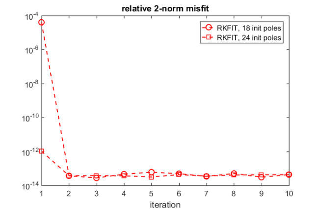
We may also initialize RKFIT with $18$ infinite initial poles, which is a convenient choice if no a priori information about the location of the poles is available.

initinf = repmat(inf, 1, 18);

% Rerun RKFIT and plot convergence.
[xi, ratfun, misfit_rkfitinf] = rkfit(F, A, b, initinf, param);
semilogy(misfit_rkfitinf, 'r*--')
xlabel('iteration')
title('relative 2-norm error')
legend('RKFIT, 18 init poles' , ...
       'RKFIT, 24 init poles',...
       'RKFIT, 18 infinite init poles');
axis([1, 10, 1e-15, 1e2])

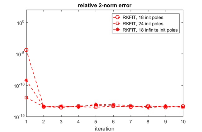
For all three choices of initial poles we find that RKFIT converges within $1$ or $2$ iterations. In fact, Corollary 3.2 in [3] asserts that RFKIT converges in a single iterations if $F$ is a rational function. It is due to the presence of rounding errors that the convergence is delayed slightly.

Comparison with vector fitting

We now compare RKFIT with the vector fitting code described in [4, 5].

The following code makes sure the vectfit3 implementation of VFIT is on MATLAB's search path, and if it is, defines some options.

if exist('vectfit3') ~= 2
  warning('Vector fitting VFIT3 not found in the Matlab path.');
  warning('VFIT can be downloaded from:')
  warning('http://www.sintef.no/Projectweb/VECTFIT/Downloads/VFUT3/')
  warning('Skipping comparison with VFIT3.');
  return
end

xi_vfit = init;    % 18 Initial poles from above
opts.relax  = 1;   % Relaxed non-triviality constraint.
opts.stable = 0;   % Do not enforce stable poles.
opts.asymp  = 3;   % Options are 1, 2, or 3.
opts.skip_pole = 0;
opts.skip_res  = 0;
opts.spy1 = 0;    opts.spy2 = 0;
opts.logx = 0;    opts.logy = 0;
opts.errplot = 0; opts.phaseplot = 0;

We now run $10$ iteration for the $18$ and $24$ finite poles used before. The VFIT implementation does not allow for infinite poles, as those would lead to Vandermonde matrices.

% Use the 18 finite poles as initial guess for VFIT.
for iter = 1:10
  [SER, xi_vfit, rmserr, fit] = ...
      vectfit3(f(zz.'), zz.', xi_vfit, b.', opts);
  misfit_vfit(iter) = norm(f(zz.') - fit)/norm(F*b);
end

ffit = @(zz) arrayfun(@(z) sum((SER.C).'./(z-diag(SER.A))) ...
                      + SER.D + z*SER.E,zz);
figure(1)
plot(abs(zz)/1e4, abs(ffit(zz)),'b:')
xlabel('imag(z)/1e4')
title('abs(function value)')
legend('exact', 'RKFIT', 'VFIT', 'Location', 'NorthWest')
figure(2), hold on
semilogy(misfit_vfit, 'bo:')
legend('RKFIT', 'VFIT')
figure(3)
plot(xi_vfit,'bx')
legend('exact poles', 'RKFIT poles', 'VFIT poles', ...
       'Location', 'NorthWest');

% Use the 24 poles as initial guess for VFIT.
xi_vfit = init24;
for iter = 1:10
  [SER, xi_vfit, rmserr, fit] = ...
      vectfit3(f(zz.'), zz.', xi_vfit, b.', opts);
  misfit_vfit24(iter) = norm(f(zz.') - fit)/norm(F*b);
end

% And plot the errors.
figure(2)
semilogy(misfit_vfit24,'bs:')
legend('RKFIT, 18 init poles', ...
       'RKFIT, 24 init poles', ...
       'RKFIT, 18 infinite init poles', ...
       'VFIT, 18 init poles', ...
       'VFIT, 24 init poles');

> In vectfit3 (line 364)
  In example_frequency (line 204)
  In evalmxdom>instrumentAndRun (line 109)
  In evalmxdom (line 21)
  In publish (line 189)
  In x_examplepublish (line 96) 
Warning: Matrix is close to singular or badly scaled. Results may be inaccurate.
RCOND =  1.463385e-16. 
> In vectfit3 (line 629)
  In example_frequency (line 204)
  In evalmxdom>instrumentAndRun (line 109)
  In evalmxdom (line 21)
  In publish (line 189)
  In x_examplepublish (line 96) 
Warning: Rank deficient, rank = 18, tol =  8.881784e-14. 
> In vectfit3 (line 364)
  In example_frequency (line 227)
  In evalmxdom>instrumentAndRun (line 109)
  In evalmxdom (line 21)
  In publish (line 189)
  In x_examplepublish (line 96) 
Warning: Matrix is close to singular or badly scaled. Results may be inaccurate.
RCOND =  3.603243e-29. 
> In vectfit3 (line 629)
  In example_frequency (line 227)
  In evalmxdom>instrumentAndRun (line 109)
  In evalmxdom (line 21)
  In publish (line 189)
  In x_examplepublish (line 96) 
Warning: Rank deficient, rank = 8, tol =  8.881784e-14. 
> In vectfit3 (line 364)
  In example_frequency (line 227)
  In evalmxdom>instrumentAndRun (line 109)
  In evalmxdom (line 21)
  In publish (line 189)
  In x_examplepublish (line 96) 
Warning: Matrix is close to singular or badly scaled. Results may be inaccurate.
RCOND =  1.617763e-16. 
> In vectfit3 (line 629)
  In example_frequency (line 227)
  In evalmxdom>instrumentAndRun (line 109)
  In evalmxdom (line 21)
  In publish (line 189)
  In x_examplepublish (line 96) 
Warning: Rank deficient, rank = 12, tol =  8.881784e-14. 
> In vectfit3 (line 364)
  In example_frequency (line 227)
  In evalmxdom>instrumentAndRun (line 109)
  In evalmxdom (line 21)
  In publish (line 189)
  In x_examplepublish (line 96) 
Warning: Matrix is close to singular or badly scaled. Results may be inaccurate.
RCOND =  1.701280e-16. 
> In vectfit3 (line 629)
  In example_frequency (line 227)
  In evalmxdom>instrumentAndRun (line 109)
  In evalmxdom (line 21)
  In publish (line 189)
  In x_examplepublish (line 96) 
Warning: Rank deficient, rank = 16, tol =  8.881784e-14. 
> In vectfit3 (line 364)
  In example_frequency (line 227)
  In evalmxdom>instrumentAndRun (line 109)
  In evalmxdom (line 21)
  In publish (line 189)
  In x_examplepublish (line 96) 
Warning: Matrix is close to singular or badly scaled. Results may be inaccurate.
RCOND =  1.749895e-16. 
> In vectfit3 (line 629)
  In example_frequency (line 227)
  In evalmxdom>instrumentAndRun (line 109)
  In evalmxdom (line 21)
  In publish (line 189)
  In x_examplepublish (line 96) 
Warning: Rank deficient, rank = 20, tol =  8.881784e-14. 
> In vectfit3 (line 629)
  In example_frequency (line 227)
  In evalmxdom>instrumentAndRun (line 109)
  In evalmxdom (line 21)
  In publish (line 189)
  In x_examplepublish (line 96) 
Warning: Rank deficient, rank = 22, tol =  8.881784e-14. 
> In vectfit3 (line 629)
  In example_frequency (line 227)
  In evalmxdom>instrumentAndRun (line 109)
  In evalmxdom (line 21)
  In publish (line 189)
  In x_examplepublish (line 96) 
Warning: Rank deficient, rank = 22, tol =  8.881784e-14. 
> In vectfit3 (line 629)
  In example_frequency (line 227)
  In evalmxdom>instrumentAndRun (line 109)
  In evalmxdom (line 21)
  In publish (line 189)
  In x_examplepublish (line 96) 
Warning: Rank deficient, rank = 22, tol =  8.881784e-14. 
> In vectfit3 (line 364)
  In example_frequency (line 227)
  In evalmxdom>instrumentAndRun (line 109)
  In evalmxdom (line 21)
  In publish (line 189)
  In x_examplepublish (line 96) 
Warning: Matrix is close to singular or badly scaled. Results may be inaccurate.
RCOND =  1.829971e-16. 
> In vectfit3 (line 629)
  In example_frequency (line 227)
  In evalmxdom>instrumentAndRun (line 109)
  In evalmxdom (line 21)
  In publish (line 189)
  In x_examplepublish (line 96) 
Warning: Rank deficient, rank = 22, tol =  8.881784e-14. 
> In vectfit3 (line 629)
  In example_frequency (line 227)
  In evalmxdom>instrumentAndRun (line 109)
  In evalmxdom (line 21)
  In publish (line 189)
  In x_examplepublish (line 96) 
Warning: Rank deficient, rank = 22, tol =  8.881784e-14. 
> In vectfit3 (line 629)
  In example_frequency (line 227)
  In evalmxdom>instrumentAndRun (line 109)
  In evalmxdom (line 21)
  In publish (line 189)
  In x_examplepublish (line 96) 
Warning: Rank deficient, rank = 22, tol =  8.881784e-14.

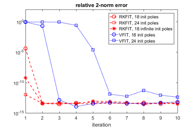
Note: The above warnings outputted by VFIT are due to ill-conditioned linear algebra problems being solved, a problem that is circumvented with RKFIT by the use of discrete-orthogonal rational basis functions.

This is the end of this example. The following creates a thumbnail.

figure(1), plot(NaN)

References

[1] M. Berljafa and S. Güttel. A Rational Krylov Toolbox for MATLAB, MIMS EPrint 2014.56 (http://eprints.ma.man.ac.uk/2390/), Manchester Institute for Mathematical Sciences, The University of Manchester, UK, 2014.

[2] M. Berljafa and S. Güttel. Generalized rational Krylov decompositions with an application to rational approximation, SIAM J. Matrix Anal. Appl., 36(2):894--916, 2015.

[3] M. Berljafa and S. Güttel. The RKFIT algorithm for nonlinear rational approximation, SIAM J. Sci. Comput., 39(5):A2049--A2071, 2017.

[4] B. Gustavsen. Improving the pole relocating properties of vector fitting, IEEE Trans. Power Del., 21(3):1587--1592, 2006.

[5] B. Gustavsen and A. Semlyen. Rational approximation of frequency domain responses by vector fitting, IEEE Trans. Power Del., 14(3):1052--1061, 1999.