Barycentric interpolation via the AAA algorithm
Steven Elsworth and Stefan GüttelDownload PDF or m-file
Contents
Introduction
Since version 2.7 the RKToolbox provides two new utility functions util_bary2rkfun and util_aaa for working with rational functions in barycentric representation
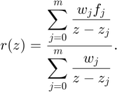
The function util_bary2rkfun takes as inputs the interpolation points (vector z), function values (vector f), and barycentric weights (vector w) of the interpolant. It then outputs the same rational function converted into RKFUN format. See [2] for details on this conversion.
The util_aaa is a wrapper for the AAA algorithm developed in [3], which appears to be a very robust method for scalar rational approximation on arbitrary discrete point sets. The only differences of util_aaa compared to the original AAA implementation in [3] are that
- the output is returned in RKFUN or RKFUNM format, using the conversion described in [2],
- it also works for a matrix-valued function F by using a scalar surrogate function
 for the AAA sampling.
A simple scalar example
In an example taken from [3, page 27] the AAA algorithm is used to compute a rational approximant  to the Riemann zeta function
  on the interval
 ![$[4 - 40i, 4 + 40i]$](example_aaa_eq13820183544021603423.png) . Here we do the same, using the util_aaa wrapper:
. Here we do the same, using the util_aaa wrapper:
zeta = @(z) sum(bsxfun(@power,(1e5:-1:1)',-z));
Z = linspace(4-40i, 4+40i);
rat = util_aaa(zeta,Z);
The computed rational approximant rat is of degree 29. As it is an object of RKFUN type we can, for example, evaluate it for matrix arguments. Following [2], we compute  for a shifted skew-symmetric matrix
  having eigenvalues in
 ![$[4 - 40i; 4 + 40i]$](example_aaa_eq11666352770684989344.png) and a vector
and a vector  . This evaluation uses the efficient rerunning algorithm described in [1, Section 5.1] and requires no diagonalization of . We then compute and display the relative error of the approximant:
A = 10*gallery('tridiag',10); S = 4*speye(10);
A = [ S , A ; -A , S ]; b = ones(20,1);
f = rat(A, b); % approximates zeta(A)*b
[V,D] = eig(full(A)); ex = V*(zeta(diag(D).').'.*(V\b));
norm(ex - f)/norm(ex)
ans =
   8.1412e-14
Solving a nonlinear eigenproblem
While the AAA algorithm is designed for scalar-valued functions  , the computed interpolants can easily be modified to interpolate matrix-valued functions
  . The util_aaa implements a surrogate approximation approach where the matrix-valued function is first reduced to with random unit vectors and then sampled via AAA. The scalar rational interpolant
  is then recast as a matrix-valued interpolant by replacing the function values
  in the barycentric formula with matrices
  .
.
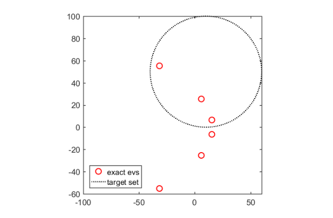
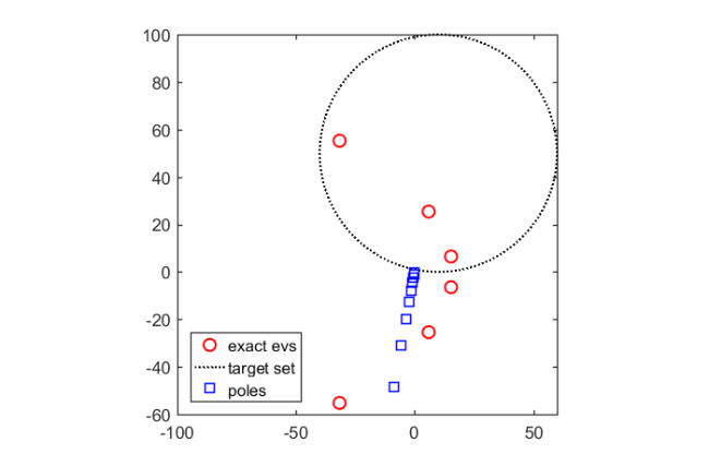
We demonstrate this procedure with the help of a simple nonlinear eigenvalue problem (NEP)  , with the matrix defined above. We choose a disk of radius 50 centered at
  as the target set, inside of which there are three eigenvalues of :
F = @(z) A - sqrt(z)*speye(20);
evs = eig(full(A)).^2; % exact eigenvalues of F
figure(1), plot(evs,'ro'); hold on; shg
Z = 10 + 50i + 50*exp(1i*linspace(0,2*pi,100));
plot(Z,'k:'); axis equal; axis([-100,60,-60,100])
legend('exact evs','target set','Location','SouthWest')
The boundary circle is discretized by 100 equispaced points, providing the set  of candidate points. We can now run util_aaa to sample this function, say with an error tolerance of
  .
.
ratm = util_aaa(F,Z,1e-12)
ratm =
	RKFUNM object of size 20-by-20 and type (14, 14).
	Complex sparse coefficient matrices of size 20-by-20.
	Complex-valued Hessenberg pencil (H, K) of size 15-by-14.
The output is an object of class RKFUNM, a  matrix-valued rational function of degree
  . Note that the error tolerance we used when calling util_aaa corresponds to the approximation error for the scalar surrogate problem, not necessarily for the matrix-valued NEP. Anyway, let's plot the poles of ratm, which appear to align on a (nonstandard) branch cut for the square root:
plot(poles(ratm),'bs')
legend('exact evs','target set','poles',...
    'Location','SouthWest')
The solution of the rational NEP is now straightforward: We simply need to linearize the RKFUNM and compute the eigenvalues of the resulting matrix pencil:
AB = linearize(ratm);
[A,B] = AB.get_matrices();
evs = eig(full(A),full(B));
plot(evs,'m+')
legend('exact evs','target set','poles','eigenvalues',...
    'Location','SouthWest')
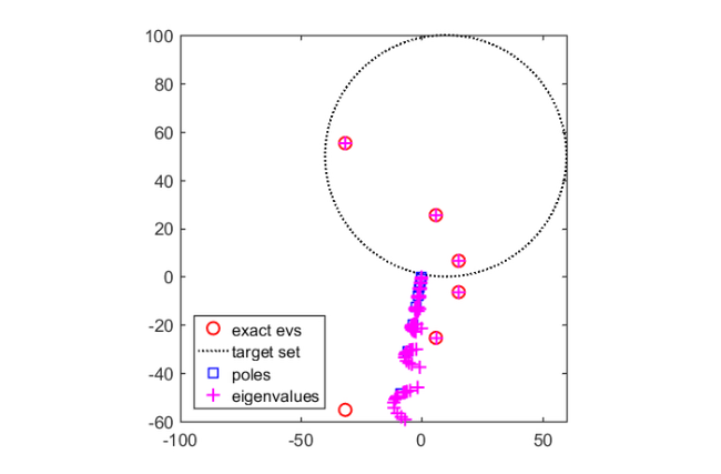
Note how the eigenvalues of the linearization are very good approximations to the eigenvalues of inside the target set. Of course, solving the linearized problem using eig as above is only viable for small problems. However, this is not a problem as the pencil structure AB can also be used as an input to the rat_krylov method. The following lines compute Ritz approximations to the eigenvalues of the linearization from a rational Krylov space of dimension  , having all shifts identically placed at the center of the target disk:
shifts = repmat(10 + 50i, 1, 15);
[m,n] = type(ratm);
dimlin = m*size(ratm,1); % dimension of linearization
v = randn(dimlin, 1);    % starting vector of Krylov space
shifts = repmat(10 + 50i, 1, 14);
[V, K, H] = rat_krylov(AB, v, shifts);
[X, D] = eig(H(1:end-1, :), K(1:end-1, :));
ritzval = diag(D);
plot(ritzval, 'g*')
legend('exact evs','target set','poles','eigenvalues',...
    'Ritz values','Location','SouthWest')
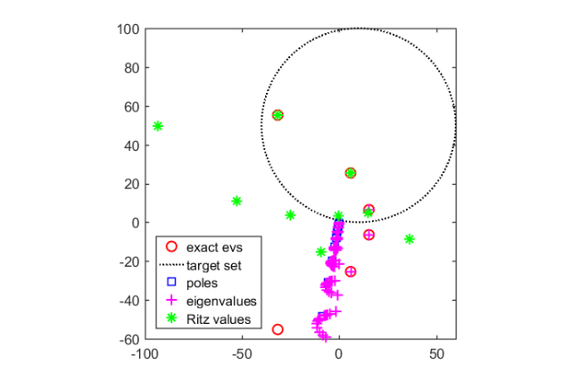
As one can see, the two Ritz values close to the center of the disk are already quite close to the desired eigenvalues. The accuracy can be increased by computing Ritz values of order higher than .
References
[1] M. Berljafa and S. Güttel. The RKFIT algorithm for nonlinear rational approximation, SIAM J. Sci. Comput., 39(5):A2049--A2071, 2017.
[2] S. Elsworth and S. Güttel. Conversions between barycentric, RKFUN, and Newton representations of rational interpolants, Linear Algebra Appl., 576:246--257, 2019.
[3] Y. Nakatsukasa, O. Sete, and L. N. Trefethen. The AAA algorithm for rational approximation, SIAM J. Sci. Comput., 40(3):A1494--A1522, 2018.