Matching centrality measures for networks

Mary Aprahamian and Stefan Güttel, March 2016Download PDF or m-file

Introduction
Power network example
Exponential centrality
Resolvent centrality
References

Introduction

The analysis of complex networks using tools from linear algebra has recently regained popularity. One way to define the relative importance of a network's node, known as centrality, is to quantify its ability to initiate walks around the network. The connection to linear algebra is that with each graph we can associate an adjacency matrix $A$ , so that $A_{ij} = 1$ if there is an edge (either directed or undirected) from $i$ to $j$ , and $A_{ij} = 0$ otherwise. The number of walks of length $k$ between nodes $i$ and $j$ is obtained as the $(i,j)$ element of $A^k$ . The total number of walks originating from node $i$ is the $i$ -th element of the vector $\sum_{k=0}^\infty A^k \mathbf{1}$ , where $\mathbf{1}$ is the vector of all ones.

In applications it may be unreasonable to weigh very short and very long walks equally, so walks of length $k$ are penalized by a parameter $0< \alpha_k \le 1$ . Two choices of $\alpha_k$ have been particularly popular: $\alpha_k = \alpha^k$ with $0<\alpha<1$ , and $\alpha_k = 1/k!$ . In the former case we assume further that $\alpha < 1/\rho(A)$ , where $\rho(A)$ is the spectral radius of $A$ . In this case the vector centrality scores are the elements of $(I-\alpha A)^{-1}\mathbf{1}$ . This resolvent-based measure is known as Katz centrality [4]. In the second case the vector of centrality scores is $\exp(A)\mathbf{1}$ . This exponential-based measure is known as total communicability [2].

Depending on the application, either the exponential centrality or the resolvent centrality may be more appropriate to rank the importance of nodes, but also computational considerations may determine the choice of centrality. An interesting question is the following: for which value of the Katz parameter $\alpha$ will both centrality measures be most similar?

This question is, of course, a simple rational approximation problem. For example, if we aim to minimize the 2-norm difference between the centrality vectors (allowing for some scaling), the problem becomes: find (real) parameters $\alpha,\beta$ such that

$\| \exp(A)\mathbf{1} - \beta (I-\alpha A)^{-1}\mathbf{1} \|_2 \to \min.$

Note that if we are only interested in the ranking of nodes, the scaling of the resolvent centralities by $\beta$ will have no effect on the ordering of the nodes.

Power network example

We now demonstrate how RKFIT [3] can be used to determine good values for $\alpha$ and $\beta$ , a problem that is equivalent to finding a type $(0,1)$ rational approximant $r(A)\mathbf{1}$ , $r(z) = \beta / (1-\alpha z)$ , of the exponential centrality $\exp(A)\mathbf{1}$ .

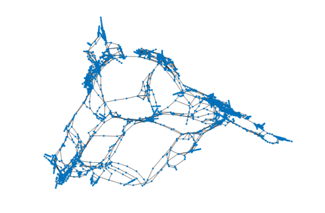
We consider a network arising as a topological representation of the Western States Power Grid of the USA. The network is available from the Florida Sparse Matrix collection (http://www.cise.ufl.edu/research/sparse/matrices/Newman/power.html). As a first step we load the adjacency matrix $A$ of the network and plot its associated graph:

if exist('power.mat') ~= 2
  disp('File power.mat not found. Can be downloaded from:')
  disp(['http://www.cise.ufl.edu/research/sparse/' ...
	'matrices/Newman/power.html'])
  return
end

load power.mat
A = Problem.A;
G = graph(A, 'OmitSelfLoops');
plot(G, 'LineWidth', 1, 'EdgeColor', [0, 0, 0]);
axis([-5.7, 7.5, -7, 6.5]), axis off

Exponential centrality

We now compute the exponential centralities using the function expmv available from http://www.mathworks.com/matlabcentral/fileexchange/29576-matrix-exponential-times-a-vector/content/expmv.m. By sorting the entries of the vector $\exp(A)\mathbf{1}$ , we can identify the 10 highest ranked nodes in the power network:

if exist('expmv') ~= 2
  disp('Code exmpv not found. Can be downloaded from:')
  disp(['http://www.mathworks.com/matlabcentral/fileexchange/' ...
	'29576-matrix-exponential-times-a-vector/content/expmv.m'])
  return
end

b = ones(size(A, 1), 1);
F = @(v) expmv(1, A, v);
centr_exp = F(b);
[~, ind_exp] = sort(centr_exp, 'descend');
disp(ind_exp(1:10))

Resolvent centrality

Now let us apply RKFIT for finding a Katz parameter $\alpha$ and the scaling $\beta$ so that the resolvent-based centrality is closest to the exponential-based centrality in the 2-norm. The residue command allows us to easily convert the found ratfun into partial fraction form, which will have a single term here:

xi = inf;  % initial guess for the pole
param = struct('real', 1, 'maxit', 5, 'k', -1);
[xi, ratfun, misfit] = rkfit(F, A, b, xi, param);
[beta, xi] = residue(ratfun);
alpha_rkfit = 1/xi;

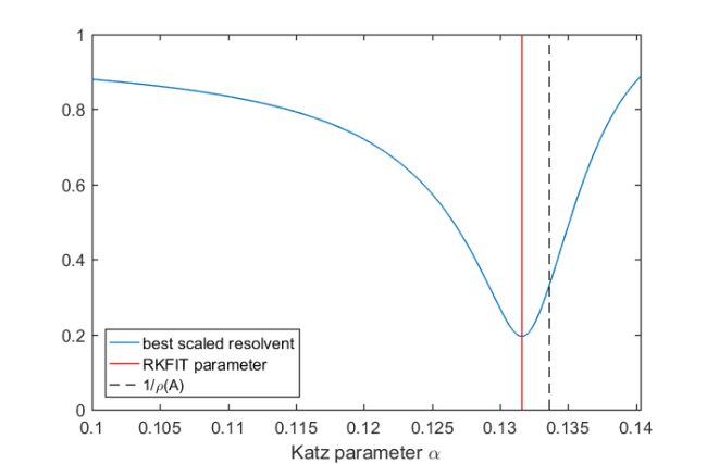
Let us investigate the error of the type (0,1) best rational approximation to the exponential centrality vector of $\exp(A)\mathbf{1}$ as we vary the parameter $\alpha$ . Note that, for given $\alpha$ , finding the optimal $\beta$ such that $\| \exp(A)\mathbf{1} - \beta (I-\alpha A)^{-1}\mathbf{1} \|_2$ is smallest possible amounts to a linear least squares problem which we can solve by projection:

rhoA = eigs(A, 1);
Alph = linspace(0.1, 1.05/rhoA, 500);
for j = 1:length(Alph),
    res = (speye(size(A)) - Alph(j)*A)\b;
    res = res/norm(res);
    beta = res'*centr_exp;
    best_approx = beta*res;
    Dist(j) = norm(centr_exp - best_approx)/norm(centr_exp);
end
figure, plot(Alph, Dist, 'LineWidth', 1), hold on
plot([alpha_rkfit, alpha_rkfit], [0, 1], 'r', 'LineWidth', 1)
plot([1/rhoA, 1/rhoA], [0, 1], 'k--', 'LineWidth', 1)
legend('best scaled resolvent', 'RKFIT parameter', ...
    '1/\rho(A)', 'Location', 'SouthWest')
xlabel('Katz parameter \alpha'), axis tight

We note that RKFIT has done a very good job in locating the minimum, called $\alpha_\mathrm{rkfit}$ . Moreover, we find that $\alpha_\mathrm{rkfit}$ also satisfies the condition on the Katz parameter to be smaller than $1/\rho(A)$ .

Another approach for choosing $\alpha$ has been suggested in [1]. There the aim was to minimize the distance between the two unscaled centrality vectors $\| \exp(A)\mathbf{1} - (I - \alpha A)^{-1}\mathbf{1} \|_2$ (i.e., $\beta=1$ ). The authors recommend a value for the Katz parameter $\alpha_\mathrm{min}$ depending on the largest eigenvalue $\rho(A)$ of the adjacency matrix, $\alpha_\mathrm{min} = (1-\exp(-\rho(A))/\rho(A)$ . For our power network the values $\alpha_\mathrm{min}$ and $\alpha_\mathrm{rkfit}$ are very close:

alpha_min = (1 - exp(-rhoA))/rhoA;
disp([ alpha_min, alpha_rkfit ])

   1.3356e-01   1.3162e-01

Here are the 15 highest ranked nodes using the exponential centrality measure and the resolvent centrality measures obtained using the parameters $\alpha_\mathrm{rkfit}$ chosen by RKFIT and $\alpha_\mathrm{min}$ suggested in [1]:

centr_rkfit = (speye(size(A)) - alpha_rkfit*A)\b;
[~, ind_rkfit] = sort(centr_rkfit, 'descend');

centr_min = (speye(size(A))-alpha_min*A)\b;
[~, ind_min] = sort(centr_min, 'descend');

[ (1:15)', ind_exp(1:15), ind_rkfit(1:15), ind_min(1:15) ]

ans =
           1        4346        4382        4382
           2        4382        4346        4346
           3        4337        4337        4337
           4        4333        4333        4333
           5        4353        4353        4353
           6        4396        4385        4385
           7        4385        4403        4403
           8        4374        4348        4348
           9        4348        4396        4396
          10        4403        4374        4374
          11        4362        4362        4399
          12        4399        4399        4362
          13        4402        4402        4402
          14        4414        4414        4414
          15        4409        4409        4409

Both parameters provide a good resolvent-based match to the exponential centrality. In fact, the nodes ranked in the top 10 using the resolvent are the same with $\alpha_\mathrm{rkfit}$ and $\alpha_\mathrm{min}$ . The first difference between these two is in the 11-th and 12-th nodes which swap their positions when $\alpha_\mathrm{min}$ is used.

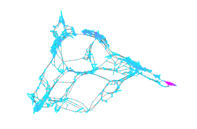
Finally, let us plot again the graph with the nodes being coloured according to the RKFIT-based centralities. Blue color indicates nodes of low centrality, and nodes with high centrality are plotted in magenta. The sizes of the nodes reflect their degrees.

figure
deg = degree(G);
plot(G, 'MarkerSize', 2*log(deg+1), ...
    'NodeCData', log(centr_rkfit), ...
    'LineWidth', 1, 'EdgeColor', [0, 0, 0]);
colormap(cool)
axis([-5.7, 7.5, -7, 6.5]), axis off

References

[1] M. Aprahamian, D. J. Higham, and N. J. Higham. Matching exponential-based and resolvent-based centrality measures, Journal of Complex Networks, 4(2):157--176, 2015.

[2] M. Benzi and C. Klymko. Total communicability as a centrality measure, Journal of Complex Networks, 1(2):124--149, 2013.

[3] M. Berljafa and S. Güttel. The RKFIT algorithm for nonlinear rational approximation, SIAM J. Sci. Comput., 39(5):A2049--A2071, 2017.

[4] L. Katz. A new status index derived from sociometric analysis, Psychometrika 18(1):39--43, 1953.