Exponential of a nonnormal matrix

Mario Berljafa and Stefan Güttel, February 2015Download PDF or m-file

Introduction
Running RKFIT with real data
Evaluating the rational approximant
Some other choices for the initial poles
References

Introduction

This is an example of RKFIT being used for approximating $\exp(A)\mathbf b$ , the action of the matrix exponential onto a vector $\mathbf b$ . RKFIT is described in [1,2] and this code reproduces Example 3 in [1].

This example demonstrates that RKFIT can sometimes find sensible approximants even when $A$ is a nonnormal and all initial poles are chosen at infinity. However, we also demonstrate that the convergence can be sensitive to the intial guess, as is not surprising with nonlinear iterations. We show how real (or complex conjugate) poles can be enforced in RKFIT.

We first define the matrix $A$ , the vector $\mathbf b$ , and the matrix $F$ corresponding to $\exp(A)$ . Our aim is then to find a rational function $r$ of type $(m,m)$ such that $\| F\mathbf b - r(A)\mathbf b \|_2$ is small.

N = 100;
A = -5*gallery('grcar', N, 3);
b = ones(N, 1);
f = @(x) exp(x); fm = @(X) expm(full(X));
F = fm(A);
exact = F*b;

[fov, evs] = util_fovals(full(A), 100);

In order to run RKFIT we only need to specify the initial poles $\xi_j$ of $r$ . In this first test let's choose all 16 initial poles equal to infinity.

m = 16;
init_xi = inf(1, m);

Running RKFIT with real data

As all quantities $F$ , $A$ , and $\mathbf b$ , as well as the initial poles are real or infinite, it is recommended to use the 'real' option. RKFIT will then attempt to produce a rational approximant with perfectly complex conjugate (or even real) poles. We set the tolerance for the relative misfit to $10^{-12}$ :

maxit = 10;
tol   = 1e-12;
xi    = init_xi;
[xi,ratfun,misfit,out] = rkfit(F,A,b,xi,maxit,tol,'real');
xi_rkfit = xi;

All computed poles appear in perfectly complex conjugate pairs.

xi_rkfit

xi_rkfit =
  Columns 1 through 2
   5.0886e+00 - 2.9517e+01i   5.0886e+00 + 2.9517e+01i
  Columns 3 through 4
   9.3538e+00 - 2.5243e+01i   9.3538e+00 + 2.5243e+01i
  Columns 5 through 6
   1.2161e+01 - 2.1323e+01i   1.2161e+01 + 2.1323e+01i
  Columns 7 through 8
   1.4113e+01 - 1.7513e+01i   1.4113e+01 + 1.7513e+01i
  Columns 9 through 10
   1.5456e+01 - 1.3717e+01i   1.5456e+01 + 1.3717e+01i
  Columns 11 through 12
   1.6329e+01 - 9.8811e+00i   1.6329e+01 + 9.8811e+00i
  Columns 13 through 14
   1.6836e+01 - 5.9754e+00i   1.6836e+01 + 5.9754e+00i
  Columns 15 through 16
   1.7062e+01 - 2.0015e+00i   1.7062e+01 + 2.0015e+00i

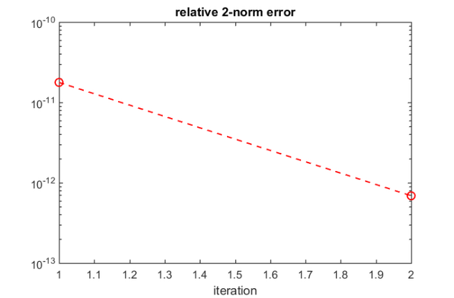
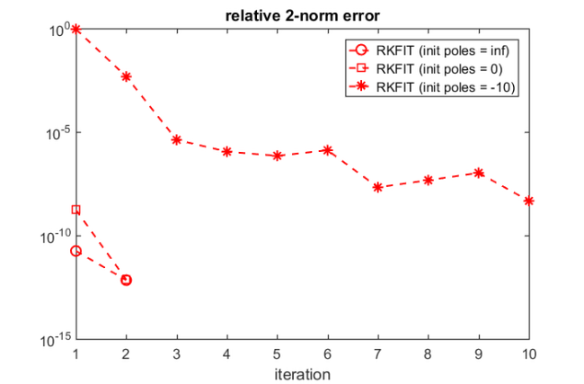
Here is a convergence history of RKFIT, showing the relative misfit defined as $\| F\mathbf b - r(A)\mathbf b \|_2/\|F \mathbf b\|_2$ at each iteration. It turns out that only two iterations were required.

figure(2)
semilogy(misfit, 'ro--')
xlabel('iteration')
title('relative 2-norm error')

Evaluating the rational approximant

The second output ratfun is an object that can be used to evaluate the computed rational approximant. This evaluation is implemented in two ways. The first option is to evaluate a matrix function $r(A)\mathbf b$ by calling ratfun(A,b) with two input arguments. For example, here we are calculating the absolute misfit:

disp(norm(F*b - ratfun(A,b)))

   3.7847e-12

Alternatively, we can evaluate $r(z)$ pointwise by giving only one input argument. Let's plot the modulus of the scalar error function 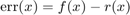$\mathrm{err}(x) = f(x) - r(x)$ over a region in the complex plane:

[X,Y] = meshgrid(linspace(-18,18,500),linspace(-30,30,500));
Z = X + 1i*Y;
E = f(Z) - ratfun(Z);
figure(1)
contourf(X,Y,log10(abs(E)),linspace(-16,8,25))
hold on
plot(evs,'r.', 'MarkerSize', 6)
plot(fov, 'm-')
plot(xi_rkfit, 'gx')
xlabel('real(z)'); ylabel('imag(z)')
title('abs(exp(z) - r(z))')
legend('error', 'evs', 'fov', 'poles', ...
       'Location', 'NorthWest')
colorbar

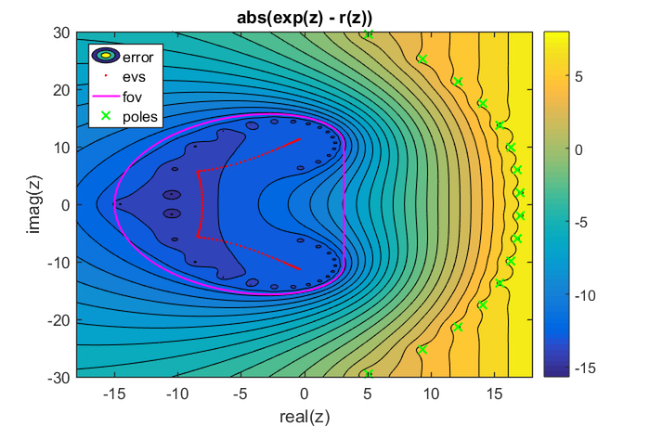
Some other choices for the initial poles

Choosing all initial poles equal to infinite seems to work fine. Let us try a finite initial guess, e.g., choosing all poles at $0$ :

init_xi = zeros(1, m);

Again, RKFIT requires only $2$ iterations:

[xi,ratfun,misfit,out] = rkfit(F,A,b,init_xi,maxit,tol,'real');
figure(2), hold on
semilogy(misfit,'rs--')
legend('RKFIT (init poles  = inf)','RKFIT (init poles = 0)')

Finally, let's change the initial poles to $-10$ . This turns out to be an unlucky initial guess and RKFIT fails to find a minimizer within $10$ iterations. Note that the matrix $A$ is highly nonnormal and RKFIT is a nonlinear iteration, which will probably make the convergence analysis of this example very involved.

init_xi = -10*ones(1, m);
[xi,ratfun,misfit,out] = rkfit(F,A,b,init_xi,maxit,tol,'real');
semilogy(misfit,'r*--')
legend('RKFIT (init poles = inf)','RKFIT (init poles = 0)',...
       'RKFIT (init poles = -10)')

That's it. The following creates a thumbnail.

figure(1), plot(NaN)

References

[1] M. Berljafa and S. Güttel. Generalized rational Krylov decompositions with an application to rational approximation, SIAM J. Matrix Anal. Appl., 36(2):894--916, 2015.

[2] M. Berljafa and S. Güttel. The RKFIT algorithm for nonlinear rational approximation, SIAM J. Sci. Comput., 39(5):A2049--A2071, 2017.