Vector autoregression via block Krylov methods
Steven Elsworth and Stefan Güttel, January 2019Download PDF or m-file
Contents
Introduction
This example reproduces Example 3.5.4 in [2], and the example in Section 7.1 in [1], using the RKFUNB framework.
Multivariate time series arise in a variety of applications including Econometrics, Geophysics, and industrial processing. The simplest type of time series model uses linear relations between the series values at successive time steps. Suppose that  (of size
  ) collects the values of
  time series at timestep
  , then using a finite number
  of past values, the vector autoregessive model VAR() is given by

where  are matrices of size
  and
and  is an
is an  vector of means. We can evaluate the quality of the model by comparing the observed values to predicted values; see [2] for details.
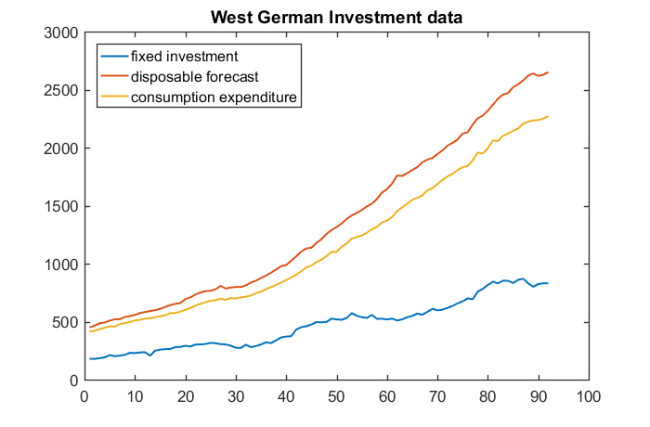
Consider the seasonally adjusted West German fixed investment, disposable income, and consumption expenditures from File E1 associated with [2]. Together these form multivariate time series  on which we perform vector autoregression. We start by importing the data and viewing the time series.
if exist('e1.dat.txt') ~= 2
   disp(['The required matrix for this problem can be '  ...
         'downloaded from http://www.jmulti.de/data_imtsa.html']);
   return
end
import = importdata('e1.dat.txt');
y = import.data;
plot(y)
title('West German Investment data')
legend('fixed investment', 'disposable forecast', 'consumption expenditure',...
    'Location', 'northwest')
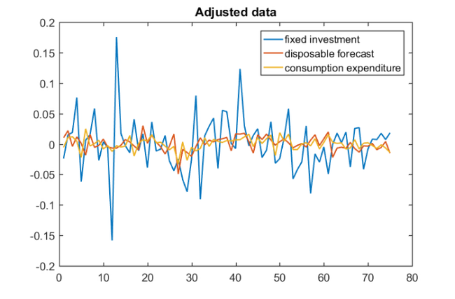
Before estimating a VAR() model, we need to make the time series stationary. Here this can be achieved by taking first-order differences of the logarithms of the data and then mean-centering. To coincide with Example 3.5.4 in [2], we also truncate the first samples of the time series before estimating the mean. For this example, we choose  .
.
y = diff(log(y));
orig_y = y;
y = y(1:75, :);
mu = mean(y(3:end,:));
y = y - ones(length(y),1)*mu;
plot(y), title('Adjusted data')
legend('fixed investment', 'disposable forecast', 'consumption expenditure')
VAR via block Krylov techniques
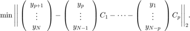
We now use least squares approximation to find the coefficients  of the vector autoregressive model. That is, we solve the minimization problem
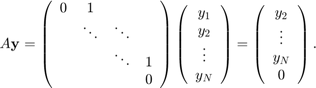
With the shift matrix
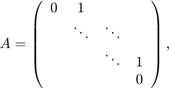
we can simulate the time evolution as left-multiplications of the  time series block vector
  by
by  :
:
The above minimization problem can hence be reformulated in terms of and , provided we define a bilinear form to trunate the last elements of the vectors. Let  diag
diag  and
and  , then our minimization problem can be written as

This problem is solved implicitly by the block rational Arnoldi method during the construction of  , the third block vector in the block-orthonormal rational Krylov basis. Furthermore, the resulting VAR(
 ) model can be represented as an RKFUNB object:
A = spdiags([zeros(size(y,1),1),ones(size(y,1),1)],0:1,size(y,1),size(y,1));
xi_ = inf*ones(1, 2);
D = zeros(75,75); D(1:73, 1:73) = eye(73);
param.balance = 0;
param.inner_product = @(x, y) y'*D*x;
[V, K, H, out] = rat_krylov(A, y, xi_, param);
R = out.R(1:3, 1:3);
C = {zeros(3), zeros(3), H(7:9, 4:6)*H(4:6, 1:3)*R};
r_ = rkfunb(K, H, C)
r_ =
	RKFUNB object of block size 3-by-3 and type (2, 2).
	Real-valued Hessenberg pencil (H, K) of size 9-by-6.
	Real dense coefficient matrices of size 3-by-3.
Using the VAR() model, we can construct one-step predictions by evaluating the RKFUNB at a smaller version of the finite shift matrix and the last two entries of the time series. The first step in the block rational Arnoldi method is to construct the QR factorisation of the initial block vector . Before evaluating the RKFUNB, we reverse this process by multiplying on the right by  .
.
Ahat = [0, 1; 0, 0];
yhat = y(end-1: end, :);
pred1 = -r_(Ahat, yhat/R);
prediction_1 = pred1(end-1,:) + mu
yhat = [yhat(2:end, :); prediction_1 - mu];
pred2 = -r_(Ahat, yhat/R);
prediction_2 = pred2(end-1,:) + mu
prediction_1 =
  -9.8600e-03   1.9912e-02   2.1857e-02
prediction_2 =
   1.1645e-02   2.0458e-02   1.4819e-02
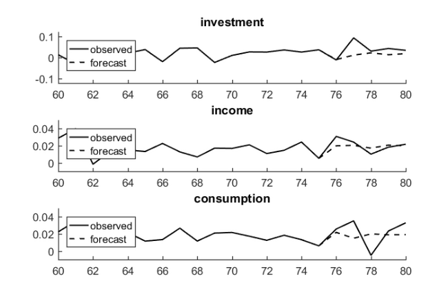
Alternatively, we can construct the VAR(2) model using explicit least squares approximation; see Section 7.1 in [1] for further details. Finally, we reproduce Fig. 3.3 in [2] by repeatedly computing one-step predictions using our RKFUNB object.
yhat = y(end-1: end, :);
predictions = [];
for i = 1:5
    pred = -r_(Ahat, yhat/R);
    predictions = [predictions; pred(end-1, :)];
    yhat = [yhat(2:end, :); pred(end-1, :)];
end
Title = {'investment', 'income', 'consumption'};
Axis = {[60, 80, -0.12, 0.12], [60, 80, -0.01, 0.05], [60, 80, -0.01, 0.05]};
for i = 1:3
    subplot(3,1,i)
    hold on
    plot(orig_y(1:80, i), 'k')
    plot(75:80, [orig_y(75, i); predictions(:, i) + mu(i)], 'k--')
    axis(Axis{i})
    title(Title{i})
    legend({'observed', 'forecast'}, 'Location', 'northwest')
end
References
[1] S. Elsworth and S. Güttel. The block rational Arnoldi method, SIAM J. Matrix Anal. Appl., 41(2):365--388, 2020.
[2] H. Lütkepohl. New Introduction to Multiple Time Series Analysis, Springer-Verlag, 2005.