Computing with rational functions

Mario Berljafa and Stefan GüttelDownload PDF or m-file

Introduction
Evaluating an rkfun
Plotting
Pole- and root-finding
Basic arithmetic operations and differentiation
Multiple precision computations
Conversion to partial fraction form
Conversion to quotient and continued fraction form
References

Introduction

This toolbox comes with an implementation of a class called rkfun, which is the fundamental data type to represent and work with rational functions. Objects of this class are produced by the rkfit function (described in [2,3]), which in its simplest use case attemts to find a rational function $r$ such that

$\|F\mathbf b - r(A)\mathbf b\|_2 \to \min,$

where $A, F$ are square matrices and $\mathbf{b}$ is a vector of compatible sizes. For example, let us consider $A = \mathrm{tridiag}(-1,2,-1)$ , $\mathbf b = [1,0,\ldots,0]^T$ , and $F = (A-2I)^2(A^2-I)^{-1} (A-4I)^{-1}$ . We know that $r(z) = (z-2)^2(z^2-1)^{-1}(z-4)^{-1}$ is a minimizer for the above problem. Let us try to find it via RKFIT:

N = 100;
A = gallery('tridiag', N);
I = speye(N);
F = (A - 4*I)\(A - 2*I)^2/(A^2 - I);
b = eye(N,1);

xi = inf(1, 5);

[xi,ratfun,misfit] = rkfit(F, A, b, xi, 5, 1e-10, 'real');

As we started with $m=5$ initial poles (at infinity), RKFIT will search for a rational function $r$ of type $(5,5)$ . When more than 1 iteration is performed and the tolerance tol is not chosen too small, RKFIT will try to reduce the type of the rational function while still maintaining a relative misfit below the tolerance, i.e., $\|F\mathbf b - r(A)\mathbf b\|_2 \leq \mathrm{tol} \|F \mathbf{b}\|_2$ . Indeed, a reduction has taken place and the type has been reduced to $(2,3)$ , as can be seen from the following output:

disp(ratfun)

	RKFUN object of type (2, 3).
	Real-valued Hessenberg pencil (H, K) of size 4-by-3.
	coeffs = [-0.087, -0.394, -1.331, -1.503]

We can now perform various operations on the ratfun object, all implemented as methods of the class rkfun. To see a list of all methods just type help rkfun. We will now discuss some methods in more detail.

Evaluating an `rkfun`

We can easily evaluate $r(z)$ at any point (or many points) in the complex plane. The following command will evaluate $r(2)$ and $r(3+\mathrm{i})$ simultaneously:

disp(ratfun([2; 3+1i]))

  -1.2226e-14 + 0.0000e+00i
   1.1765e-02 - 1.5294e-01i

We can also evaluate $r$ as a matrix function, i.e., computing $r(M)B$ for matrices $M$ and $B$ , by using two input arguments. For example, by setting $B=I$ we effectively compute the full matrix function $r(M)$ :

M = [3, 1; 0, 3];
B = eye(2);
R = ratfun(M, B)

R =
  -1.2500e-01  -2.8125e-01
            0  -1.2500e-01

Plotting

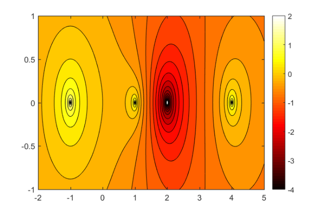
As $r$ can be evaluated at any point in the complex plane, it is straightforward to produce plots of this function. For example, here is a contour plot of $\log_{10} |r|$ over the complex region $[-2,5]\times [-1,1]i$ :

figure(1)
[X,Y] = meshgrid(-2:.01:5, -1:.01:1);
Z = X + 1i*Y;
R = ratfun(Z);
contourf(X, Y, log10(abs(R)), -4:.25:2)
colormap hot, colorbar

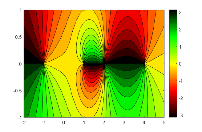
The following plot shows the phase portrait of $r$ on the same domain. Can you spot the three poles and a double root?

figure(3)
contourf(X, Y, angle(R), 20)
set(gca,'CLim',[-pi,+pi])
colormap(util_colormapc(1, 90));
colorbar

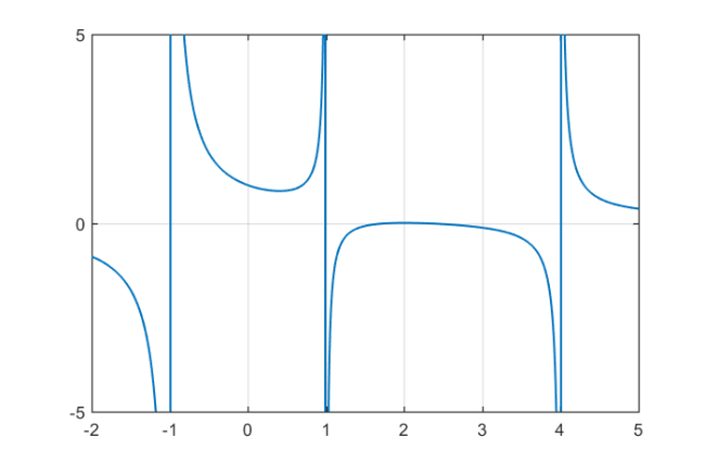
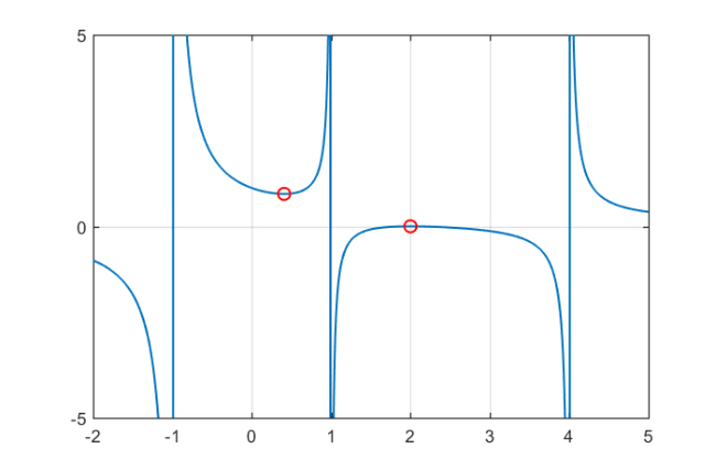
Another command ezplot can be used to get a quick idea of how ratfun looks over an interval on the real axis, in this case, $[-2,5]$ :

figure(2)
ezplot(ratfun, [-2, 5])
ylim([-5, 5])
grid on

Pole- and root-finding

From the above plot we guess that $r$ has poles at $x=\pm 1$ and $x=4$ and a root at $x=2$ , which is to be expected from the definition of $r$ . The two commands poles and roots do exactly what their names suggest:

pls = poles(ratfun)
rts = roots(ratfun)

pls =
  -1.0000e+00
   1.0000e+00
   4.0000e+00
rts =
   2.0000e+00 + 2.7597e-07i
   2.0000e+00 - 2.7597e-07i

As expected from a type (2,3) rational function, there are two roots and three poles. Note that the pole at $x=-1$ is identified with slightly less accuracy than the poles at $x=1$ and $x=4$ . This is because the point $x=-1$ is outside the spectral interval of $A$ and hence sampled less accurately. Also the double root at $x=2$ is identified up to an accuracy of $\approx 10^{-7}$ only. This is not surprising as the function is flat nearby multiple roots. However, the backward error of the roots is small:

disp(ratfun(rts))

   4.9960e-16 + 1.0588e-22i
   4.9960e-16 - 1.0588e-22i

Basic arithmetic operations and differentiation

We have implemented some very basic operations for the rkfun class, namely, the multiplication by a scalar and the addition of a scalar. The result of such operations is again an rkfun object. For example, the following command computes points $z$ where $2 r(z) = \pi$ :

z = roots(2*ratfun - pi)
disp(ratfun(z))

z =
  -4.0504e-01
   8.5769e-01
   1.5708e+00
   1.5708e+00

We have currently not implemented the summation and multiplication of two rkfun objects, though this is doable in principle. ---UPDATE: This is no longer the case since Version 2.2 of the toolbox. Check out the example on "Electronic filter design using RKFUN arithmetic".--- However, we can already differentiate a rational function using the diff command. The following will find all real local extrema of $r$ by computing the real roots of $r'$ :

extrema = roots(diff(ratfun),'real')

extrema =
   4.0759e-01
   2.0000e+00

There are two real extrema which we can add to the above plot of $r$ :

figure(2), hold on
plot(extrema, ratfun(extrema), 'ro')

The syntax and "feel" of these computations is inspired by the Chebfun system [4], which represents polynomials via Chebyshev interpolants and allows for many more operations to be performed than our rkfun implementation. Here we are representing rational functions through their coefficients in a discrete-orthogonal rational function basis. Working with rational functions poses some challenges not encountered with polynomials. For example, the indefinite integral of a rational function is not necessarily a rational function but may contain logarithmic terms.

Multiple precision computations

Objects of class rkfun can be converted to MATLAB's Variable Precision Arithmetic (VPA) as follows:

disp(vpa(ratfun))

	RKFUN object of type (2, 3).
	Real-valued Hessenberg pencil (H, K) of size 4-by-3.
	Variable precision arithmetic (VPA) activated.
	coeffs = [-0.087, -0.394, -1.331, -1.503]

Alternatively, we can also use the Advanpix Multiple Precision (MP) toolbox [1], which is typically more efficient and reliable than VPA. We recommend the use of this toolbox in particular for high-precision root-finding of rkfun's and conversion to partial fraction form:

ratfun = mp(ratfun)

ratfun = 
	RKFUN object of type (2, 3).
	Real-valued Hessenberg pencil (H, K) of size 4-by-3.
	Multiple precision arithmetic (ADVANPIX) activated.
	coeffs = [-0.087, -0.394, -1.331, -1.503]

When evaluating a multiple precision ratfun, the result will be returned in multiple precision:

format longe
ratfun(2)

ans = 
    -1.2125294919816719385880796519441591e-14

It is important to understand that, although the evaluation of ratfun is now done in multiple precision, the computation of ratfun using the rkfit command has been performed in standard double precision. rkfit does not currently support the computation of rkfun objects in multiple precision. Here are the roots of ratfun computed in multiple precision:

roots(ratfun)

ans = 
Columns 1 through 1
        2.00000000000005884325215506037004691e+00 +     2.69725359428640320019961191862469502e-07i    
        2.00000000000005884325215506037004691e+00 -     2.69725359428640320019961191862469502e-07i

Conversion to partial fraction form

It is often convenient to convert a rational function $r$ into its partial fraction form

$\displaystyle r(z) = \alpha_0 + \frac{\alpha_1}{z-\xi_1} + \cdots + \frac{\alpha_m}{z-\xi_m}.$

The residue command of our toolbox performs such a conversion. Currently, this only works when the poles $\xi_j$ of $r$ are distinct and $r$ is not of superdiagonal type (i.e., there is no linear term in $r$ ). As the conversion to partial fraction form can be an ill-conditioned transformation, we recommend to use residue in conjunction with the multiple precision feature. Here are the poles $\xi_j$ and residues $\alpha_j$ ( $j=1,\ldots,m$ ), as well as the absolute term $\alpha_0$ , of the function $r$ defined above:

[alpha, xi, alpha0, cnd] = residue(mp(ratfun));
double([xi , alpha])
double(alpha0)

ans =
    -9.999999999999628e-01     8.999999999998803e-01
     9.999999999999993e-01    -1.666666666666714e-01
     3.999999999999999e+00     2.666666666666091e-01
ans =
    -1.749809464778146e-17

The absolute term is close to zero because $r$ is of subdiagonal type. The output cnd of residue corresponds to the condition number of the transformation to partial fraction form. In this case of a low-order rational function with well separated poles the condition number is actually quite moderate:

cnd

cnd =
     5.615057038451497e+01

Conversion to quotient and continued fraction form

Our toolbox also implements the conversion of a rkfun to quotient form $r = p/q$ with two polynomials $p$ and $q$ given in the monomial basis. As with the conversion to partial fraction form, we recommend performing this transformation in multiple precision arithmetic due to potential ill-conditioning. Here we convert $r$ into the $p/q$ form and evaluate it at the root $x=2$ using MATLAB's polyval command:

[p,q] = poly(double(ratfun));
polyval(p, 2)./polyval(q, 2)

ans =
    -1.273055734903527e-14

A rkfun can also be converted into continued fraction form

$$ \displaystyle r(z) = h_0 + \cfrac{1}{\hat h_1+\cfrac{1}{h_1+\cfrac{1}{\hat h_2+\cdots+\cfrac{1}{h_{m-1}+\cfrac{1}{\hat h_m z+\cfrac{1}{h_m}}}}}} $$

as follows:

[h, hhat, absterm, cnd] = contfrac(mp(ratfun));

That's it for this tutorial. Note that more methods will be added over time and we'd be happy to receive any feedback or bug reports. For more details about the internal representation of rkfun, see [3].

The following command creates a thumbnail.

figure(3), hold on, plot(NaN)

References

[1] Advanpix LLC., Multiprecision Computing Toolbox for MATLAB, ver 4.3.3.12213, Tokyo, Japan, 2017. http://www.advanpix.com/.

[2] M. Berljafa and S. Güttel. Generalized rational Krylov decompositions with an application to rational approximation, SIAM J. Matrix Anal. Appl., 36(2):894--916, 2015.

[3] M. Berljafa and S. Güttel. The RKFIT algorithm for nonlinear rational approximation, SIAM J. Sci. Comput., 39(5):A2049--A2071, 2017.

[4] T. A. Driscoll, N. Hale, and L. N. Trefethen. Chebfun Guide, Pafnuty Publications, Oxford, 2014. http://www.chebfun.org