CD player model order reduction
Steven Elsworth and Stefan Güttel, January 2019Download PDF or m-file
Contents
Introduction
Consider a linear time invariant multi-input multi-output system described by the state space equations
and

where  denotes the state vector of length
  and
and  denote the input and output vectors of length
  . The large sparse matrix
  is of size
  and
and  are of size
  .
.
Block rational Krylov spaces [2] are a powerful tool for model order reduction provided a good set of poles is chosen. Here we explore different choices of poles, and compare how well the the reduced model behaves compared to the original system.
CD player
We start by loading the CD player problem, and constructing a function handle for the transfer function of the system:
For each set of poles, we construct the approximate transfer function

We compare the two models by plotting the error
for  over the range of
 ![$i [10^0, 10^6]$](example_cdplayer_eq04057575525140290626.png) .
.
if exist('CDplayer.mat') ~= 2
   disp(['The required matrix for this problem can be downloaded from '  ...
         'http://slicot.org/20-site/126-benchmark-examples-for-model-reduction']);
   return
end
load CDplayer
H = @(s) C*((s*speye(size(A)) - A)\B);
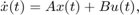
Infinite poles vs equally spaced poles
We compare a block polynomial Krylov approximation against a block rational Krylov approximation. The polynomial space is constructed with 10 poles set to infinity, whereas the rational space has 5 poles logarithmically spaced in the interval ![$i[10^0, 10^6]$](example_cdplayer_eq14464304135779436376.png) , complemented with their complex conjugates to obtain a real block rational Arnoldi decomposition. For both approaches, we plot the norm of the difference between the transfer function and the approximate tranfer function.
, complemented with their complex conjugates to obtain a real block rational Arnoldi decomposition. For both approaches, we plot the norm of the difference between the transfer function and the approximate tranfer function.
% block polynomial Krylov space
xi = inf*ones(1,10);
V = rat_krylov(A,B,xi);

Am = V'*A*V;
Cm = C*V;
Bm = V'*B;
Hm = @(s) Cm*((s*speye(size(Am)) - Am)\Bm);
Xm = @(s) V*((s*eye(size(Am)) - Am)\(V'*B));
Gam = @(s) B - (s*speye(size(A)) - A)*Xm(s);

errHm = [];
s = 1i*logspace(0,6,500);
for k = 1:length(s)
   errHm(k) = norm(H(1i*s(k)) - Hm(1i*s(k)));
end

loglog(imag(s), errHm, 'LineWidth',2); hold on
xlabel('frequency $\omega$', 'Interpreter', 'latex')
ylabel('$\|H(i \omega) - H_m(i \omega)\|_2$', 'Interpreter', 'latex')

% block rational Krylov space
xi = 1i*logspace(0,6,5);
xi = util_cplxpair(xi, conj(xi));
param.real = 1;
V = rat_krylov(A,B,xi);

Am = V'*A*V;
Cm = C*V;
Bm = V'*B;
Hm = @(s) Cm*((s*speye(size(Am)) - Am)\Bm);

errHm = [];
s = union(xi, 1i*logspace(0,6,500));
for k = 1:length(s)
   errHm(k) = norm(H(s(k)) - Hm(s(k)));
end

p = loglog(imag(xi), ones(1, length(xi)), 'kx', 'MarkerSize', 12);
loglog(imag(s), errHm, 'LineWidth',2); axis([0, 1e6, 1e-6, 1e6])
xlabel('frequency $\omega$', 'Interpreter', 'latex')
ylabel('$\|H(i \omega) - H_m(i \omega)\|_2$', 'Interpreter', 'latex')
legend({'polynomial', 'poles', 'rational'})
Adaptive pole selection
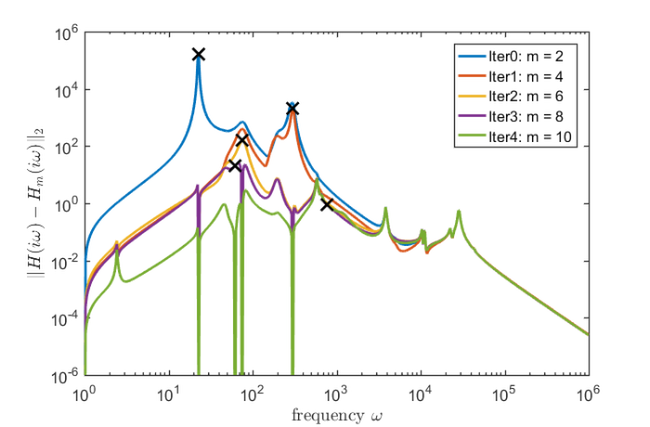
In this example we start with two poles at ![$[1i, -1i]$](example_cdplayer_eq15954124589738281418.png) . We then select the following poles adaptively, in complex conjugate pairs, using the procedure described in Section 3.2 in [1]. This procedure proves to be quite effective, with the error curve dropping significantly from iteration to iteration. Note that we are using the extension functionality of the rat_krylov function, which allows to extend an existing block rational Arnoldi decomposition with new block basis vectors.
. We then select the following poles adaptively, in complex conjugate pairs, using the procedure described in Section 3.2 in [1]. This procedure proves to be quite effective, with the error curve dropping significantly from iteration to iteration. Note that we are using the extension functionality of the rat_krylov function, which allows to extend an existing block rational Arnoldi decomposition with new block basis vectors.
cand = 1i*logspace(0,6,500);
xi = [ 1i , conj(1i) ];
param.real = 1;
[V, K_, H_] = rat_krylov(A, B, xi, param); % initial run

param.extend = 2;  % allow for the iterative extension of BRAD
figure()
for iter = 1:5
    Am = V'*A*V;
    Bm = V'*B;
    Cm = C*V;
    Hm = @(s) Cm*((s*speye(size(Am)) - Am)\Bm);
    Xm = @(s) V*((s*eye(size(Am)) - Am)\(V'*B));
    Gam = @(s) B - (s*speye(size(A)) - A)*Xm(s);
    errHm = [];
    for k = 1:length(cand)
        nrmGam(k) = norm(Gam(cand(k)));
        errHm(k) = norm(H(cand(k)) - Hm(cand(k)));
    end
    mem(iter)=loglog(imag(cand),errHm, 'LineWidth',2);
    hold on, shg

    [val,ind] = max(nrmGam);
    loglog(imag(cand(ind)), errHm(ind), 'kx', 'MarkerSize', 12, 'LineWidth', 2)
    xi = [ cand(ind) , conj(cand(ind)) ];
    [V,K_,H_] = rat_krylov(A, V, K_, H_, xi, param); % extend decomposition
end

legend(mem,{'Iter0: m = 2', 'Iter1: m = 4', 'Iter2: m = 6', ...
    'Iter3: m = 8', 'Iter4: m = 10'})
xlabel('frequency $\omega$', 'Interpreter', 'latex')
ylabel('$\|H(i \omega) - H_m(i \omega)\|_2$', 'Interpreter', 'latex')
axis([0, 1e6, 1e-6, 1e6])
References
[1] O. Abidi, M. Hached, and K. Jbilou. Adaptive rational block Arnoldi methods for model reductions in large-scale MIMO dynamical systems, New Trends Math. Sci., 4(2):227--239, 2016
[2] S. Elsworth and S. Güttel. The block rational Arnoldi method, SIAM J. Matrix Anal. Appl., 41(2):365--388, 2020.