The parallel rational Arnoldi algorithm
Mario Berljafa and Stefan GüttelDownload PDF or m-file
Contents
Introduction
Since version 2.4 of the RKToolbox, the rat_krylov function can simulate the parallel construction of a rational Krylov basis. This is done by imposing various nonzero patterns in a so-called continuation matrix  . Simply speaking, the
  -th column of this matrix contains the coefficients of the linear combination of rational Krylov basis vectors which have been used to compute the next
  -th basis vector. Therefore is an upper triangular matrix.
Parallelization strategies
By imposing certain nonzero patters on the continuation matrix , we can simulate a parallel rational Arnoldi algorithm where several linear system solves are performed synchronously. Note that the typically most expensive part in the rational Arnoldi algorithm is the solution of large linear systems of equations, hence parallelizing this component can yield significant savings in computation time.
There are various continuation strategies (i.e., ways to form the matrix ), each with a different numerical behaviour, and we refer to [1] for an overview. By default, the strategy ruhe is used, which determines the next admissible continuation vector (column of ) by computing a QR factorization of a small matrix [2]. Other available parallelization strategies are last, almost-last, and near-optimal.
The strategy almost-last is the one used by Skoogh [3]. The near-optimal strategy is the one developed and advocated in [1]. It uses a (cheap) predictor method to anticipate the direction of the next Krylov basis vector(s) in order to determine a good continuation matrix . By "good" we mean that the rational Krylov basis that is orthogonalized is well-conditioned, so that numerical instabilities in the Gram--Schmidt process are limited.
Basic usage
We now demonstrate at a simple example how to use the parallel option in rat_krylov. Links to the practically relevant examples are given below.
First, let us define a matrix  , a starting vector
  , and a sequence of pole parameters, where
  consecutive poles are pairwise distinct. Having distinct poles is a necessary requirement for parallelization.
load west0479
A  = west0479;
b  = ones(479,1);
xi = repmat([-50, -25, 25, 50], 1, 4);
Now we can run rat_krylov to compute a rational Arnoldi decomposition 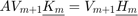 , with the basis vectors in
  being generated in parallel. This is done by specifying the continuation strategy and the p = 4 parameter:
param = struct('continuation', 'almost-last', ...
               'p',            4,             ...
               'orth',         'CGS',         ...
               'reorth',       1,             ...
               'waitbar',      1 );

[V, K, H, out] = rat_krylov(A, b, xi, param);
The other struct fields specify that classical Gram-Schmidt orthogonalization has been used with reorthogonalization, the columns of the matrix pencil  have been rescaled in an attempt to improve the numerical conditioning, and a waitbar has been displayed during the computation.
The output parameter out has several fields of interest, in particular, it returns the continuation matrix being used during the computation. Here is a spy plot of :
spy(out.T)
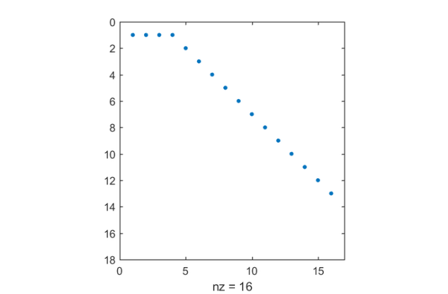
We can clearly see how Skoogh's almost-last strategy works: in every parallel cycle, rational Krylov basis vectors are computed, each from the last vector obtained on the respective parallel process in the previous parallel cycle.
The output parameter out.R corresponds to the  factor in the implicitly computed QR factorization of the rational Krylov basis. As is explained in much more detail in [1], its condition number is an indicator for the stability of the computation. We observe that with the almost-last strategy this condition number is rather high:
R = out.R;
D = fminsearch(@(x) cond(R*diag(x)), ones(size(R, 2), 1), ...
               struct('Display','off'));
disp(cond(R*diag(D)))
3.2177e+06
Near-optimal continuation strategy
To overcome, or at least reduce, the numerical problems observed with canonical parallelization strategies (such as almost-last and last), rat_krylov implements the near-optimal strategy suggested in [1]. With this strategy, a (cheap) predictor method is used to anticipate the direction of rational Krylov basis vectors before their actual computation, to infer good continuation pairs.
param.continuation = 'near-optimal';
[V, K, H, out] = rat_krylov(A, b, xi, param);
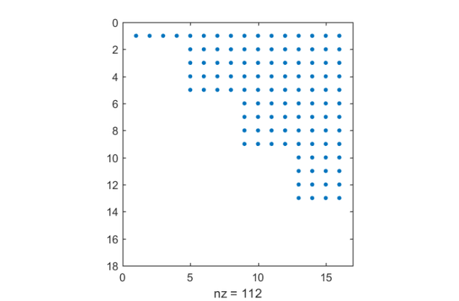
The continuation matrix has a more dense pattern compared to the almost-last strategy, but still allows for basis vectors to be computed in parallel:
spy(out.T)
The condition number of the basis being orthogonalized is significantly smaller:
R = out.R;
D = fminsearch(@(x) cond(R*diag(x)), ones(size(R, 2), 1), ...
               struct('Display','off'));
disp(cond(R*diag(D)))
5.5275e+00
In fact, this basis is so close to being orthogonal, that running classical Gram-Schmidt without orthogonalization would be fine.
The near-optimal method implemented in this simple manner is, however, computationally expensive: in fact every linear system in the rational Arnoldi algorithm has been solved twice using backslash. In a high-performance implementation one would reuse existing LU factors, or switch to an inexact predictor method like, e.g., FOM or GMRES. The predictor method is specified by a function handle in the continuation_solve field and the number of iterations is specified in continuation_m. Demonstrations of this are given in the numerical examples linked below.
Links to numerical examples
The numerical examples in [1] can be reproduced with the following scripts:
Numerical illustration from [1, Sec. 3.4]
TEM example from [1, Sec. 5.1]
Inlet example from [1, Sec. 5.2]
Waveguide example from [1, Sec. 5.3]
References
[1] M. Berljafa and S. Güttel. Parallelization of the rational Arnoldi algorithm, SIAM J. Sci. Comput., 39(5):S197--S221, 2017.
[2] A. Ruhe. Rational Krylov: A practical algorithm for large sparse nonsymmetric matrix pencils, SIAM J. Sci. Comput., 19(5):1535--1551, 1998.
[3] D. Skoogh. A parallel rational Krylov algorithm for eigenvalue computations, in G. Goos et al., editors, Applied Parallel Computing, volume 1541 of Lecture Notes in Computer Science, pages 521--526. Springer-Verlag, Berlin, 1998.