Electronic filter design using RKFUN arithmetic

Mario Berljafa and Stefan GüttelDownload PDF or m-file

Introduction
The RKFUN gallery
The symbolic constructor
Arithmetic operations with rational functions
Constructing rational filters
Limitations
References

Introduction

With Version 2.2 of the RKToolbox the rkfun class and its methods have been substantially extended. It is now possible to perform basic arithmetic operations on rational functions that go beyond scalar multiplication and addition of constants. For example, one can now add, multiply, divide, or exponentiate rkfun objects. Composition of an rkfun with a Moebius transform is also possible. Furthermore, the rkfun constructor now comes with the option to construct an object from a symbolic expression, or a string specifying a rational function from the newly introduced gallery. We now demonstrate some of these features. An application to electronic filter design is given below.

The RKFUN gallery

The rkfun class provides a gallery function which allows for the quick construction of some useful rational functions. A list of the functions currently implemented can be obtained by typing:

help rkfun.gallery

  GALLERY    Collection of rational functions.
 
  obj = rkfun.gallery(funname, param1, param2, ...) takes 
  funname, a case-insensitive string that is the name of 
  a rational function family, and the family's input 
  parameters. 
 
  See the listing below for available function families.
 
  constant   Constant function of value param1.
  cheby      Chebyshev polynomial (first kind) of degree param1.
  cayley     Cayley transformation (1-z)/(1+z).
  moebius    Moebius transformation (az+b)/(cz+d) with 
             param1 = [a,b,c,d].
  sqrt       Zolotarev sqrt approximation of degree param1 on 
             the positive interval [1,param2].
  invsqrt    Zolotarev invsqrt approximation of degree param1 on 
             the positive interval [1,param2].
  sqrt0h     balanced Remez approximation to sqrt(x+(h*x/2)^2)
             of degree param3 on [param1,param2], 
             where param1 <= 0 <= param2 and h = param4.
  sqrt2h     balanced Zolotarev approximation to sqrt(x+(hx/2)^2)
             of degree param5 on [param1,param2]U[param3,param4], 
             param1 < param2 < 0 < param3 < param4, h = param6.
  invsqrt2h  balanced Zolotarev approximation to 1/sqrt(x+(hx/2)^2)
             of degree param5 on [param1,param2]U[param3,param4], 
             param1 < param2 < 0 < param3 < param4, h = param6.
  sign       Zolotarev sign approximation of degree 2*param1 on
             the union of [1,param2] and [-param2,-1].
  step       Unit step function approximation for [-1,1] of 
             degree 2*param1 with steepness param2.

For example, we can construct an rkfun corresponding to a Moebius transform $r(z) = (4z + 3)/(2z - 1)$ as follows:

r = rkfun.gallery('moebius', [4, 3, 2, -1])

r = 
	RKFUN object of type (1, 1).
	Real-valued Hessenberg pencil (H, K) of size 2-by-1.
	coeffs = [0.000, 1.000]

As always with rkfun objects, we can perform several computations on r, such as computing its roots and poles:

format long e
disp([roots(r) poles(r)])

    -7.500000000000000e-01     5.000000000000000e-01

The symbolic constructor

Symbolic strings can also be used to construct rkfun objects, provided that the required MATLAB symbolic toolboxes are installed. Here we construct an rkfun corresponding to the rational function $s(z) = 3(z-3)(z^2-1)/(z^{5}+1)$ :

s = rkfun('3*(z-3)*(z^2-1)/(z^5+1)')

s = 
	RKFUN object of type (2, 4).
	Real-valued Hessenberg pencil (H, K) of size 5-by-4.
	coeffs = [0.000, 0.000, -0.000, -0.000, 23.570]

This works by first finding the roots and poles of the input function symbolically and then constructing the rkfun with these roots and poles numerically. Note that s is only of type $(2,4)$ as one of the five denominator roots has been cancelled out by symbolic simplifications prior to the numerical construction. The constructor should issue an error if the provided string fails to be parsed by the symbolic engine, or if it does not represent a rational function.

Arithmetic operations with rational functions

Since Version 2.2 of the RKToolbox one can add, multiply, divide, and exponentiate rkfun objects. All these operations are implemented via transformations on generalized rational Krylov decompositions [1, 2]. For example, here is the product of the two rational functions $r$ and $s$ from above:

disp(r.*s)

	RKFUN object of type (3, 5).
	Real-valued Hessenberg pencil (H, K) of size 6-by-5.
	coeffs = [0.000, 0.000, 0.000, -0.000, -0.000, ...]

Note that it is necessary to use point-wise multiplication .*, not the matrix-multiplication operator *. This is to be consistent with the MATLAB notation, and also with the notation used in the Chebfun system [5] (where the * operator returns the inner product of two polynomials; something we have not yet implemented for rkfun objects).

It is also possible to compose rkfun objects as long as the inner function is a Moebius transform, i.e., a rational function of type at most $(1,1)$ . The rational function $r$ from above is a Moebius transform, hence we can form the function $f(z) = s(r(z))^{-1}$ :

f = 1./s(r)

f = 
	RKFUN object of type (4, 4).
	Real-valued Hessenberg pencil (H, K) of size 5-by-4.
	coeffs = [-0.000, -0.002, -0.000, -0.005, -0.042]

The roots of $f$ should correspond to the poles of $s(r)$ , which are the poles of $s$ mapped under the inverse function $r^{-1}$ . The latter inverse function is indeed well defined in the whole complex plane as $r$ is an invertible Moebius transform. We can compute it via the inv command. Let's verify that the roots/poles agree numerically:

rts = sort(roots(f));
pls = sort(feval(inv(r), poles(s)));
disp([rts, pls])

  Column 1
     -4.256702311079903e-01 - 3.812725100682988e-01i
     -4.256702311079903e-01 + 3.812725100682988e-01i
     -1.187966132528373e+00 - 8.330610885153919e-01i
     -1.187966132528373e+00 + 8.330610885153919e-01i
  Column 2
     -4.256702311079903e-01 - 3.812725100682988e-01i
     -4.256702311079903e-01 + 3.812725100682988e-01i
     -1.187966132528373e+00 - 8.330610885153928e-01i
     -1.187966132528373e+00 + 8.330610885153928e-01i

Constructing rational filters

Rational filter functions are ubiquitous in scientific computing and engineering. For example, in signal processing [3, 6] one is interested in deriving rational functions that act as filters on selected frequency bands. Using the gallery of the RKToolbox and some rkfun transformations, we can construct meaningful rational filters in just a few lines of MATLAB code. Below is a plot of four popular filter types, which are obtained by rational transforms of Chebyshev polynomials or the step function from rkfun's gallery.

x = rkfun;
butterw = 1./(1 + x.^16);
cheby   = rkfun('cheby',8);
cheby1  = 1./(1 + 0.1*cheby.^2);
cheby2  = 1./(1 + 1./(0.1*cheby(1./x).^2));
ellip   = rkfun('step');

figure
subplot(221),ezplot(butterw,[0,2]);    title('Butterworth')
subplot(222),ezplot(cheby1, [0,2],'r');title('Chebyshev type 1')
subplot(223),ezplot(cheby2, [0,2],'g');title('Chebyshev type 2')
subplot(224),ezplot(ellip,  [0,2],'m');title('Elliptic')

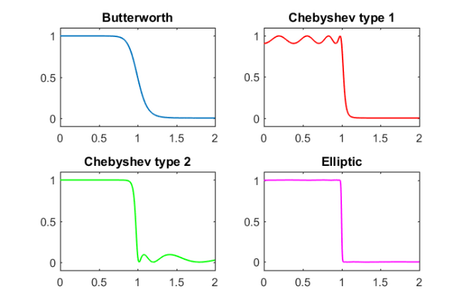
The reader may compare this plot with that at the bottom of the Wikipedia page on electronic filters [7]. For example, the filter cheby2 involves multiple inverses of a Chebyshev polynomial in the transformed variable $x \mapsto x^{-1}$ . It has the so-called equiripple property in the stopband, which is the region where the filter value is close to zero. The elliptic filter ellip, also known as Cauer filter [4], has equiripple properties in both the stop- and passbands. Such filters are based on Zolotarev's equioscillating rational functions [8], which are also implemented in the gallery of the RKToolbox.

Limitations

Although we hope that the new rkfun capabilities demonstrated above are already useful for many practical purposes, there are still some short-comings one has to be aware of. The main problem is that combinations of rkfun objects may have degrees higher than theoretically necessary, which may lead to an unnecessarily fast growth of parameters. For example, when subtracting an rkfun from itself,

r = rkfun('(1-x)/(1+x)');
d = r - r

d = 
	RKFUN object of type (2, 2).
	Real-valued Hessenberg pencil (H, K) of size 3-by-2.
	coeffs = [0.000, -1.000, 1.000]

we currently obtain a type $(2,2)$ rational function, instead of the expected type $(0,0)$ . This is because the sum (or difference) of two type $(1,1)$ rational functions is of type $(2,2)$ in the worst case, and we currently do not perform any degree reduction on the sum (or difference). (A similar problem is encountered with multiplication or division.) The roots and poles of the function d are meaningless, but the evaluation works fine, except when we evaluate at (or nearby) a "legacy" pole:

d([-1, -1+1e-16, 0, 1, 2])

ans =
  Columns 1 through 3
                         0                       NaN     2.465190328815662e-31
  Columns 4 through 5
                         0    -1.850371707708596e-17

A numerical degree reduction would probably require the concept of a "domain of evaluation." To illustrate, consider the rational function $r(z) = \frac{10^{-14}}{z} + \frac{1}{z-1}$ . The exact type of this function is $(1,2)$ , but the residue associated with $z=0$ is tiny, so one may conclude that this pole could be removed. However, when evaluating $r$ for $z\approx 0$ , the removal of this pole would lead to an inaccurate result (try $z = 10^{-14}$ ). Hence, reliable degree reduction may only be possible when a relevant "domain of evaluation" is specified.

References

[1] M. Berljafa and S. Güttel. Generalized rational Krylov decompositions with an application to rational approximation, SIAM J. Matrix Anal. Appl., 36(2):894--916, 2015.

[2] M. Berljafa and S. Güttel. The RKFIT algorithm for nonlinear rational approximation, SIAM J. Sci. Comput., 39(5):A2049--A2071, 2017.

[3] H. Blinchikoff and A. Zverev. Filtering in the Time and Frequency Domains, John Wiley & Sons Inc., New York, 1976.

[4] W. Cauer. Ein Interpolationsproblem mit Funktionen mit positivem Realteil, Math. Z., 38(1):1-44, 1934.

[5] T. A. Driscoll, N. Hale, and L. N. Trefethen. Chebfun Guide, Pafnuty Publications, Oxford, 2014. http://www.chebfun.org

[6] M. Van Valkenburg. Analog Filter Design, Holt, Rinehart and Winston, 1982.

[7] Wikipedia, entry Electronic filter as of 17/09/2015. https://goo.gl/vkQwWG

[8] E. I. Zolotarev. Application of elliptic functions to questions of functions deviating least and most from zero, Zap. Imp. Akad. Nauk St. Petersburg, 30:1-59, 1877. In Russian.