Moving the poles of a rational Krylov space

Mario Berljafa and Stefan Güttel, June 2015Download PDF or m-file

Contents

Rational Krylov spaces

A rational Krylov space is a linear vector space of rational functions in a matrix times a vector [5]. Let $A$ be a square matrix of size $N\times N$, $\mathbf{b}$ an $N\times 1$ nonzero starting vector, and let $\xi_1,\xi_2,\ldots,\xi_m$ be a sequence of complex or infinite poles all distinct from the eigenvalues of $A$. Then the rational Krylov space of order $m+1$ associated with $A,\mathbf{b},\xi_j$ is defined as

$\displaystyle \mathcal{Q}_{m+1}\equiv\mathcal{Q}_{m+1}(A,\mathbf{b}, q_m) = q_m(A)^{-1} \mathrm{span} \{ \mathbf{b},A\mathbf{b},\ldots,A^m \mathbf{b}\},$

where $q_m(z) = \prod_{{j=1,\xi_j\neq \infty}}^m (z - \xi_j)$ is the common denominator of the rational functions associated with $\mathcal{Q}_{m+1}$. The rational Krylov sequence method by Ruhe [5] computes an orthonormal basis $V_{m+1}$ of $\mathcal{Q}_{m+1}$. The first column of $V_{m+1}$ can be chosen as $V_{m+1}\mathbf e_1 = \mathbf{b}/\|\mathbf{b}\|_2$. The basis matrix $V_{m+1}$ satisfies a rational Arnoldi decomposition of the form

$\displaystyle A V_{m+1} \underline{K_m} = V_{m+1} \underline{H_m},$

where $(\underline{H_m},\underline{K_m})$ is an (unreduced) upper Hessenberg pencil of size $(m+1)\times m$.

The poles of a rational Krylov space

Given a rational Arnoldi decomposition of the above form, it can be shown [1] that the poles $\xi_j$ of the associated rational Krylov space are the generalized eigenvalues of the lower $m\times m$ subpencil of $(\underline{H_m},\underline{K_m})$. Let us verify this at a simple example by first constructing a rational Krylov space associated with the $m=5$ poles $-1,\infty,-\mathrm{i},0,\mathrm{i}$. The matrix $A$ is of size $N=100$ and chosen as the tridiag matrix from MATLAB's gallery, and $\mathbf{b}$ is the first canonical unit vector. The rat_krylov command is used to compute the quantities in the rational Arnoldi decomposition:

N  = 100;
A  = gallery('tridiag', N);
b  = eye(N, 1);
m  = 5;
xi = [-1, inf, -1i, 0, 1i];
[V, K, H] = rat_krylov(A, b, xi);

Indeed, the rational Arnoldi decomposition is satisfied with a residual norm close to machine precision:

format shorte
disp(norm(A*V*K - V*H) / norm(H))

   3.5143e-16

And the chosen poles $\xi_j$ are the eigenvalues of the lower $m\times m$ subpencil:

disp(eig(H(2:m+1,1:m),K(2:m+1,1:m)))

  -1.0000e+00 + 0.0000e+00i
          Inf + 0.0000e+00i
   0.0000e+00 - 1.0000e+00i
   0.0000e+00 + 0.0000e+00i
   0.0000e+00 + 1.0000e+00i

Moving the poles explicitly

There is a direct link between the starting vector $\mathbf{b}$ and the poles $\xi_j$ of a rational Krylov space $\mathcal{Q}_{m+1}$. A change of the poles $\xi_j$ to $\breve \xi_j$ can be interpreted as a change of the starting vector from $\mathbf{b}$ to $\mathbf{\breve b}$, and vice versa. Algorithms for moving the poles of a rational Krylov space are described in [1] and implemented in the functions move_poles_expl and move_poles_impl.

For example, let us move the poles of the above rational Krylov space $\mathcal{Q}_{m+1}$ to the points $-1,-2,\ldots,-5$:

xi_new = -1:-1:-5;
[KT, HT, QT, ZT] = move_poles_expl(K, H, xi_new);

The output of move_poles_expl are unitary matrices $Q$ and $Z$, and transformed upper Hessenberg matrices $\underline{\breve K_m} = Q\underline{K_m} Z$ and $\underline{\breve H_m} = Q\underline{H_m} Z$, so that the lower $m\times m$ part of the pencil $(\underline{\breve H_m},\underline{\breve K_m})$ has as generalized eigenvalues the new poles $\breve \xi_j$:

disp(eig(HT(2:m+1,1:m),KT(2:m+1,1:m)))

  -1.0000e+00 + 0.0000e+00i
  -2.0000e+00 + 1.4085e-15i
  -3.0000e+00 - 7.2486e-16i
  -4.0000e+00 + 1.6407e-16i
  -5.0000e+00 - 2.4095e-16i

Defining $\breve V_{m+1} = V_{m+1} Q^*$, the transformed rational Arnoldi decomposition is

$\displaystyle A \breve V_{m+1} \underline{\breve K_m} = \breve V_{m+1} \underline{\breve H_m}.$

This can be verified numerically by looking at the residual norm:

VT = V*QT';
disp(norm(A*VT*KT - VT*HT) / norm(HT))

   6.8004e-16

It should be noted that the function move_poles_expl can be used to move the $m$ poles to arbitrary locations, including to infinity, and even to the eigenvalues of $A$. In latter case, the transformed space $\breve V_{m+1}$ does not correspond to a rational Krylov space generated with starting vector $\breve V_{m+1}\mathbf e_1$ and poles $\breve \xi_j$, but must be interpreted as a filtered rational Krylov space. Indeed, the pole relocation problem is very similar to that of applying an implicit filter to the rational Krylov space [3,4]. See also [1] for more details.

Moving the poles implicitly

Assume we are given a nonzero vector $\mathbf{\breve b}\in\mathcal{Q}_{m+1}$ with coefficient representation $\mathbf{\breve b} = V_{m+1}\mathbf{c}$, where $\mathbf{c}$ is a vector with $m+1$ entries. The function move_poles_impl can be used to obtain a transformed rational Arnoldi decomposition with starting vector $\mathbf{\breve b}$.

As an example, let us take $\mathbf{c} = [0,\ldots,0,1]^T$ and hence transform the rational Arnoldi decomposition so that $\breve V_{m+1}\mathbf{e}_1 = \mathbf{v}_{m+1}$, the last basis vector in $V_{m+1}$:

c = zeros(m+1,1); c(m+1) = 1;
[KT, HT, QT, ZT] = move_poles_impl(K, H, c);
VT = V*QT';

The poles of the rational Krylov space with the modified starting vector can again be read off as the generalized eigenvalues of the lower $m\times m$ part of $(\underline{\breve H_m},\underline{\breve K_m})$:

disp(eig(HT(2:m+1,1:m),KT(2:m+1,1:m)))

   3.2914e+00 - 5.5756e-02i
   1.8705e+00 - 1.2100e-01i
   7.7852e-01 - 9.2093e-02i
   1.9752e-01 - 3.0824e-02i
   4.4392e-03 - 3.5884e-04i

This implicit pole relocation procedure is key element of the RKFIT algorithm described in [1,2].

Some fun with moving poles

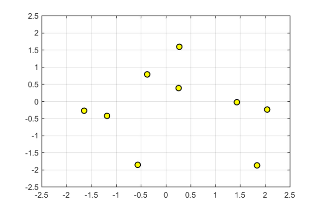
To conclude this example, let us consider a $10\times 10$ random matrix $A$, a random vector $\mathbf{b}$, and the corresponding $6$-dimensional rational Krylov space with poles at $-2,-1,0,1,2$:

A  = (randn(10) + 1i*randn(10))*.5;
b  = randn(10,1) + 1i*randn(10,1);
m  = 5;
xi = -2:2;
[V, K, H] = rat_krylov(A, b, xi);

Here are the eigenvalues of $A$:

figure
plot(eig(A),'ko','MarkerFaceColor','y')
axis([-2.5,2.5,-2.5,2.5]), grid on, hold on

We now consider a $t$-dependent coefficient vector $\mathbf{c}(t)$ such that $V_{m+1}\mathbf{c}(t)$ is continuously "morphed" from $\mathbf{v}_1$ to $\mathbf{v}_2$. The poles of the rational Krylov space with the transformed starting vector $V_{m+1}\mathbf{c}(t)$ are then plotted as a function of $t$.

for t = linspace(1,2,51),
  c = zeros(m+1,1);
  c(floor(t))   = cos(pi*(t-floor(t))/2);
  c(floor(t)+1) = sin(pi*(t-floor(t))/2);
  [KT, HT, QT] = move_poles_impl(K, H, c);% transformed pencil
  xi_new = sort(eig(HT(2:m+1,1:m),KT(2:m+1,1:m))); % new poles
  plot(real(xi_new), imag(xi_new), 'b+')
end

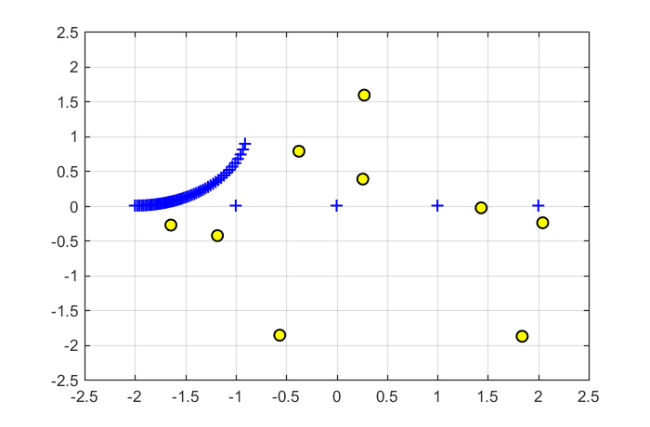
As one can see, only one of the five poles starts moving away from $-2$, with the remaining four poles staying at their positions. This is because "morphing" the starting vector from $\mathbf{v}_1$ to $\mathbf{v}_2$ only affects a two-dimensional subspace of $\mathcal{Q}_{m+1}$ which includes the vector $\mathbf{b}$ and is itself a rational Krylov space, and this space is parameterized by one pole only.

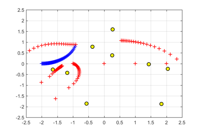
As we now continue morphing from $\mathbf{v}_2$ to $\mathbf{v}_3$, another pole starts moving:

for t = linspace(2,3,51),
  c = zeros(m+1,1);
  c(floor(t))   = cos(pi*(t-floor(t))/2);
  c(floor(t)+1) = sin(pi*(t-floor(t))/2);
  [KT, HT, QT, ZT] = move_poles_impl(K, H, c);
  xi_new = sort(eig(HT(2:m+1,1:m),KT(2:m+1,1:m)));
  plot(xi_new, 'r+')
end

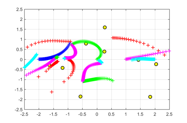
Morphing from $\mathbf{v}_3$ to $\mathbf{v}_4$, then to $\mathbf{v}_5$, and finally to $\mathbf{v}_6$ will eventually affect all five poles of the rational Krylov space:

for t = linspace(3, 5.99, 150)
  c = zeros(m+1,1);
  c(floor(t))   = cos(pi*(t-floor(t))/2);
  c(floor(t)+1) = sin(pi*(t-floor(t))/2);
  [KT, HT, QT, ZT] = move_poles_impl(K, H, c);
  xi_new = sort(eig(HT(2:m+1, 1:m), KT(2:m+1, 1:m)));
  switch floor(t)
   case 3, plot(xi_new', 'g+')
   case 4, plot(xi_new', 'm+')
   case 5, plot(xi_new', 'c+')
  end
end

References

[1] M. Berljafa and S. Güttel. Generalized rational Krylov decompositions with an application to rational approximation, SIAM J. Matrix Anal. Appl., 36(2):894--916, 2015.

[2] M. Berljafa and S. Güttel. The RKFIT algorithm for nonlinear rational approximation, SIAM J. Sci. Comput., 39(5):A2049--A2071, 2017.

[3] G. De Samblanx and A. Bultheel. Using implicitly filtered RKS for generalised eigenvalue problems, J. Comput. Appl. Math., 107(2):195--218, 1999.

[4] G. De Samblanx, K. Meerbergen, and A. Bultheel. The implicit application of a rational filter in the RKS method, BIT, 37(4):925--947, 1997.

[5] A. Ruhe. Rational Krylov: A practical algorithm for large sparse nonsymmetric matrix pencils, SIAM J. Sci. Comput., 19(5):1535--1551, 1998.

Published with MATLAB® R2016a