Square root of a symmetric matrix
Mario Berljafa and Stefan Güttel, June 2015Download PDF or m-file
Contents
Introduction
This is an example of RKFIT [1, 2, 3] being used for approximating  , the action of the matrix square root onto a vector
  . RKFIT is described in [2, 3] and implemented in the RK Toolobox [1]. This code reproduces the example from [2, Section 5.2]. We also compare RKFIT to the vector fitting code VFIT3. Vector fitting is described in [4, 5].
We first define the matrix  , the vector , and the matrix
  corresponding to
  . Our aim is then to find a rational function
  of type
  such that
  .
.
N = 500;
A = gallery('tridiag',N);
b = eye(N,1);
f = @(x) sqrt(x); fm = @(X) sqrtm(full(X));
F = fm(A);
exact = F*b;

[U, D] = eig(full(A)); ee = diag(D).';
Running rkfit
In order to run RKFIT we only need to specify the initial poles of  . In this example we pretend to not know that a reasonable choice of initial poles is on the negative real axis (the branch cut of
  ) and choose 16 infinite poles
  . As all quantities , , and , as well as the initial poles are real, it is advised running RKFIT with the 'real' option. This will attempt to produce a rational approximant with perfectly complex conjugate (or even real) poles. We perform
  RKFIT iterations.
m = 16;
[xi, ratfun, misfit] = rkfit(F, A, b, inf(1, m), 10, 'real');
It turns out that all computed poles are real negative:
disp(reshape(xi, 4, 4))
  -1.5658e+02  -9.9810e-01  -5.7343e-02  -2.2792e-03
  -1.6253e+01  -4.8662e-01  -2.7196e-02  -8.4426e-04
  -5.1139e+00  -2.4033e-01  -1.2509e-02  -2.5196e-04
  -2.1389e+00  -1.1824e-01  -5.5140e-03  -4.3750e-05
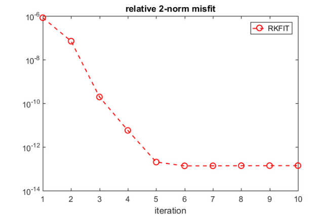
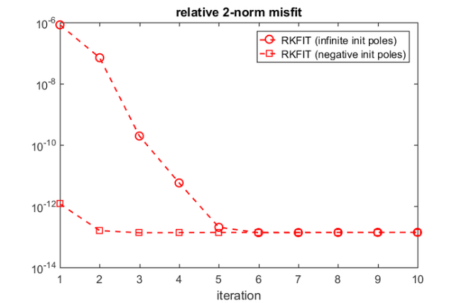
Here is a convergence plot of RKFIT, showing the relative misfit  at each iteration.
figure(1)
semilogy(misfit, 'ro--')
xlabel('iteration'), title('relative 2-norm misfit')
legend('RKFIT')
Evaluating the rational approximant
The second output ratfun is an object that can be used to evaluate the computed rational approximant. This evaluation is implemented in two ways. The first option is to evaluate a matrix function  by calling ratfun(A,b) with two input arguments. For example, here we are calculating the absolute misfit or :
disp(norm(F*b - ratfun(A, b)))
1.9306e-13
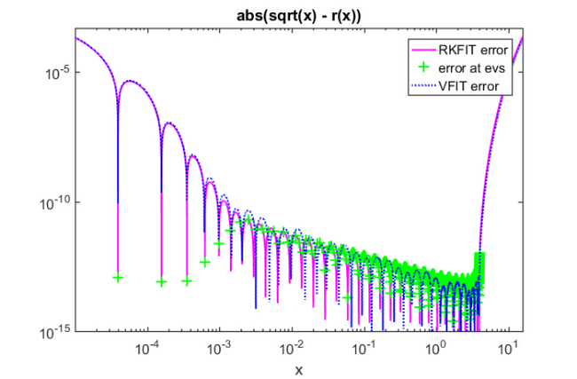
Alternatively, we can evaluate pointwise by giving only one input argument. Let us plot the modulus of the scalar error function  over the spectral interval of , which is approximately
 ![$[0,4]$](example_sqrtm_eq06167377142463551117.png) .
.
figure(2)
xx = sort([logspace(-6,log10(15.728), 5000), ee ]);
errf = f(xx) - ratfun(xx);
loglog(xx,abs(errf), 'm-')
hold on
errf = f(ee) - ratfun(ee);
loglog(ee,abs(errf), 'g+')
xlabel('x'), title('abs(sqrt(x) - r(x))')
legend('RKFIT error','error at evs')
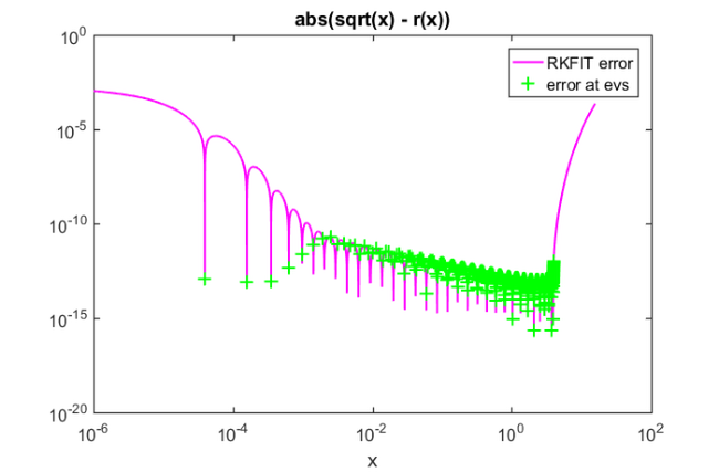
How often does this error function change sign on (or rather on the discretisation set xx, which was chosen very fine with 5000 points)? Equivalently, how many interpolation points are there?
sc = length(find(diff(sign(errf))));
disp(['The error function has ' num2str(sc) ' sign changes on [0,4].'])
The error function has 32 sign changes on [0,4].
Some different choices for the initial poles
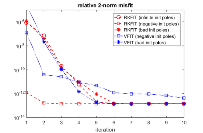
Choosing all initial poles equal to infinity seemed to work fine. Of course we can achieve convergence in fewer iterations by choosing negative initial poles, e.g., logarithmically spaced on the negative real axis. Let us rerun RKFIT with the new initial poles and compare the convergence.
tmp = -logspace(-8, 8, m);
[xi, ratfun, misfit] = rkfit(F, A, b, tmp, 10, 'real');
figure(1), hold on
semilogy(misfit, 'rs--')
legend('RKFIT (infinite init poles)', ...
       'RKFIT (negative init poles)')
Now let us try a very bad choice for the initial poles, which is to place them right into the spectral interval of :
tmp = linspace(0, 4, m);
[xi, ratfun, misfit] = rkfit(F, A, b, tmp, 10, 'real');
semilogy(misfit, 'r*--')
legend('RKFIT (infinite init poles)', ...
       'RKFIT (negative init poles)', ...
       'RKFIT (bad init poles)')
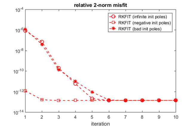
In this example, RKFIT is not very affected by the choice of the initial poles and converges robustly.
Comparison with vector fitting
We now compare RKFIT with the vector fitting code described in [4, 5].
The following code makes sure the vectfit3 implementation of VFIT is on MATLAB's search path, and if it is, defines some options.
if exist('vectfit3') ~= 2
  warning('Vector fitting VFIT3 not found in the Matlab path.');
  warning('VFIT can be downloaded from:')
  warning('http://www.sintef.no/Projectweb/VECTFIT/Downloads/VFUT3/')
  warning('Skipping comparison with VFIT3.');
  return
end

xi = -logspace(-8, 8, m);
opts.relax  = 1;   % Relaxed non-triviality constraint.
opts.stable = 0;   % Do not enforce stable poles.
opts.asymp  = 2;   % Options are 1, 2, or 3.
opts.skip_pole = 0;
opts.skip_res  = 0;
opts.spy1 = 0;    opts.spy2 = 0;
opts.logx = 0;    opts.logy = 0;
opts.errplot = 0; opts.phaseplot = 0;
For VFIT3 we need interpolation nodes and weights, and in this example these need to be chosen as the eigenvalues of and the components of in the eigenvector basis of , respectively.
Note: The below warnings outputted by VFIT are due to ill-conditioned linear algebra problems being solved, a problem that is circumvented with RKFIT by the use of discrete-orthogonal rational basis functions.
nodes = diag(D); nodes = nodes(:).';
fvals = f(nodes);
weights = U'*b; weights = weights(:).';

for iter = 1:10
  [SER, xi, rmserr, fit] = ...
      vectfit3(fvals, nodes, xi, weights, opts);
  err_vfit(iter) = norm((fvals - fit).*weights)/norm(exact);
end

figure(1)
semilogy(err_vfit,'bs:')
legend('RKFIT (infinite init poles)','RKFIT (negative init poles)',...
       'RKFIT (bad init poles)','VFIT (negative init poles)')
axis([1, 10, 1e-14, 1e-5])

ffit = @(zz) arrayfun(@(z) ...
                      sum((SER.C).'./(z-diag(SER.A))) + ...
                      SER.D + z*SER.E,zz);
figure(2)
loglog(xx,abs(f(xx) - ffit(xx)), 'b:')
axis([1e-5, 15.7, 1e-15, 5e-4])
set(gca, 'XTick', 10.^(-5:1))
legend('RKFIT error', 'error at evs', 'VFIT error')
> In vectfit3 (line 364)
  In example_sqrtm (line 166)
  In evalmxdom>instrumentAndRun (line 109)
  In evalmxdom (line 21)
  In publish (line 189)
  In x_examplepublish (line 96)
Warning: Matrix is close to singular or badly scaled. Results may be inaccurate.
RCOND =  1.721665e-16.
> In vectfit3 (line 629)
  In example_sqrtm (line 166)
  In evalmxdom>instrumentAndRun (line 109)
  In evalmxdom (line 21)
  In publish (line 189)
  In x_examplepublish (line 96)
Warning: Rank deficient, rank = 14, tol =  2.220446e-13.
> In vectfit3 (line 364)
  In example_sqrtm (line 166)
  In evalmxdom>instrumentAndRun (line 109)
  In evalmxdom (line 21)
  In publish (line 189)
  In x_examplepublish (line 96)
Warning: Matrix is close to singular or badly scaled. Results may be inaccurate.
RCOND =  1.699030e-16.
> In vectfit3 (line 629)
  In example_sqrtm (line 166)
  In evalmxdom>instrumentAndRun (line 109)
  In evalmxdom (line 21)
  In publish (line 189)
  In x_examplepublish (line 96)
Warning: Rank deficient, rank = 15, tol =  2.220446e-13.
> In vectfit3 (line 364)
  In example_sqrtm (line 166)
  In evalmxdom>instrumentAndRun (line 109)
  In evalmxdom (line 21)
  In publish (line 189)
  In x_examplepublish (line 96)
Warning: Matrix is close to singular or badly scaled. Results may be inaccurate.
RCOND =  1.912200e-16.
> In vectfit3 (line 629)
  In example_sqrtm (line 166)
  In evalmxdom>instrumentAndRun (line 109)
  In evalmxdom (line 21)
  In publish (line 189)
  In x_examplepublish (line 96)
Warning: Rank deficient, rank = 16, tol =  2.220446e-13.
> In vectfit3 (line 364)
  In example_sqrtm (line 166)
  In evalmxdom>instrumentAndRun (line 109)
  In evalmxdom (line 21)
  In publish (line 189)
  In x_examplepublish (line 96)
Warning: Matrix is close to singular or badly scaled. Results may be inaccurate.
RCOND =  2.001267e-16.
> In vectfit3 (line 629)
  In example_sqrtm (line 166)
  In evalmxdom>instrumentAndRun (line 109)
  In evalmxdom (line 21)
  In publish (line 189)
  In x_examplepublish (line 96)
Warning: Rank deficient, rank = 16, tol =  2.220446e-13.
> In vectfit3 (line 364)
  In example_sqrtm (line 166)
  In evalmxdom>instrumentAndRun (line 109)
  In evalmxdom (line 21)
  In publish (line 189)
  In x_examplepublish (line 96)
Warning: Matrix is close to singular or badly scaled. Results may be inaccurate.
RCOND =  1.527542e-16.
> In vectfit3 (line 629)
  In example_sqrtm (line 166)
  In evalmxdom>instrumentAndRun (line 109)
  In evalmxdom (line 21)
  In publish (line 189)
  In x_examplepublish (line 96)
Warning: Rank deficient, rank = 16, tol =  2.220446e-13.
> In vectfit3 (line 364)
  In example_sqrtm (line 166)
  In evalmxdom>instrumentAndRun (line 109)
  In evalmxdom (line 21)
  In publish (line 189)
  In x_examplepublish (line 96)
Warning: Matrix is close to singular or badly scaled. Results may be inaccurate.
RCOND =  1.716169e-16.
> In vectfit3 (line 629)
  In example_sqrtm (line 166)
  In evalmxdom>instrumentAndRun (line 109)
  In evalmxdom (line 21)
  In publish (line 189)
  In x_examplepublish (line 96)
Warning: Rank deficient, rank = 16, tol =  2.220446e-13.
> In vectfit3 (line 364)
  In example_sqrtm (line 166)
  In evalmxdom>instrumentAndRun (line 109)
  In evalmxdom (line 21)
  In publish (line 189)
  In x_examplepublish (line 96)
Warning: Matrix is close to singular or badly scaled. Results may be inaccurate.
RCOND =  2.203797e-16.
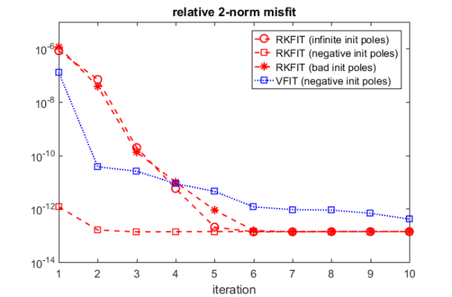
And the same with the "bad" initial poles.
xi = linspace(0, 4, m);
for iter = 1:10
  [SER, xi, rmserr, fit] = ...
      vectfit3(fvals, nodes, xi, weights, opts);
  err_vfit(iter) = norm((fvals - fit).*weights)/norm(exact);
end
figure(1)
semilogy(err_vfit, 'b*:')
legend('RKFIT (infinite init poles)', ...
       'RKFIT (negative init poles)', ...
       'RKFIT (bad init poles)',      ...
       'VFIT (negative init poles)',  ...
       'VFIT (bad init poles)')
This is the end of this example. The following creates a thumbnail.
figure(2), plot(NaN)

References
[1] M. Berljafa and S. Güttel. A Rational Krylov Toolbox for MATLAB, MIMS EPrint 2014.56 (http://eprints.ma.man.ac.uk/2390/), Manchester Institute for Mathematical Sciences, The University of Manchester, UK, 2014.
[2] M. Berljafa and S. Güttel. Generalized rational Krylov decompositions with an application to rational approximation, SIAM J. Matrix Anal. Appl., 36(2):894--916, 2015.
[3] M. Berljafa and S. Güttel. The RKFIT algorithm for nonlinear rational approximation, SIAM J. Sci. Comput., 39(5):A2049--A2071, 2017.
[4] B. Gustavsen. Improving the pole relocating properties of vector fitting, IEEE Trans. Power Del., 21(3):1587--1592, 2006.
[5] B. Gustavsen and A. Semlyen. Rational approximation of frequency domain responses by vector fitting, IEEE Trans. Power Del., 14(3):1052--1061, 1999.