Compressing exterior Helmholtz problems: Uniform approximation on indefinite interval

Stefan Güttel, October 2016Download PDF or m-file

Introduction
The code
Conclusions
Other examples
References

Introduction

This script reproduces Example 6.3 in [1]. It computes RKFIT approximants for $f(A)\mathbf{b}$ , where $A$ is a diagonal matrix with dense eigenvalues in an indefinite interval and 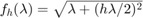$f_h(\lambda) = \sqrt{\lambda + (h\lambda/2)^2}$ . The RKFIT approximants are compared to balanced Remez approximants for the indefinite intervals.

The code

a1 = -225;  % spectral interval bounds from the 2D Laplacian example
b1 = -1e-2;
a2 = 1e-2;
b2 = 1.7976e+05;

ee = real([ logspace(log10(a1),-16,100) , logspace(-16,log10(b2),100) ]).';
N = length(ee);
A = spdiags(ee,0,N,N);
h = 1/150; h =0;
v = [ 0 , 0 ];
ex = @(x) sqrt(x + (h*x/2).^2);
F = spdiags(ex(ee),0,N,N);
b = ones(N,1); b = b/norm(b);

Initialize RKFIT parametes.

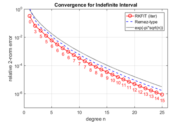
param = struct;
param.reduction = 0;
param.k = 1; % superdiagonal
param.tol = 0;
param.real = 0;

for m = 1:25,

    % run rkfit with training vector
    param.maxit = 30;
    xi = inf*ones(1,m-1); % take m-1 initial poles
    [xi,ratfun,misfit,out] = rkfit(F,A,b,xi,param);
    if m==1,
        err_rkfit = out.misfit_initial; iter_rkfit = 0;
    else
        err_rkfit(m) = min(misfit);
        iter_rkfit(m) = find(misfit <= 1.01*min(misfit),1);
    end

    % uniform balanced Remez approximant
    zolo = rkfun('sqrt0h',a1,b2,m);
    err_zolo(m) = norm(zolo(ee(:)).*b - F*b)/norm(F*b);

    if m == 10,  % some plots for m = 10

        % get best ratfun
        [~,it] = min(misfit);
        param.maxit = it;
        xi = inf*ones(1,m-1); % take m-1 initial poles
        [xi,ratfun,misfit,out] = rkfit(F,A,b,xi,param);

        figure
        semilogy(NaN); hold on
        lint = util_log2lin([b1,a2],[a1,b1,a2,b2],.1);
        fill([lint(1:2),lint([2,1])], [1e-25,1e-25,1e15,1e15], ...
            .85*[1,1,1], 'LineStyle', '-')
        ylim([1e-8,10])
        ax = [ -10.^(5:-2:-3) , 0 , 10.^(-3:2:5) ];
        linax = util_log2lin(ax,[a1,b1,a2,b2],.1);
        set(gca,'XTick',linax,'XTickLabel',ax)

        xx = [ -logspace(log10(-a1),log10(-b1),1000) , linspace(b1,a2,200) , ...
            logspace(log10(a2),log10(b2),1000) ];
        xx = union(xx,ee);
        xxt = util_log2lin(xx.',[a1,b1,a2,b2],.1).';
        eet = util_log2lin(ee.',[a1,b1,a2,b2],.1).';
        hdl1 = semilogy(xxt,abs(ratfun(xx) - ex(xx)),'r-'); hold on
        hdl2 = semilogy(xxt,abs(zolo(xx) - ex(xx)),'b--');
        legend([hdl1,hdl2],'RKFIT','Remez-type ')

        xlim([0,1]), ylim([1e-5,1e-0])
        title(['Error Curve, n = ' num2str(m) ])
        grid on, set(gca,'layer','top')
        ax = [ -10.^(2:-2:-2)  , 10.^(-2:2:5) ];
        linax = util_log2lin(ax,[a1,b1,a2,b2],.1);
        set(gca,'XTick',linax,'XTickLabel',ax)

        % plot residues
        figure
        [resid,xi] = residue(mp(ratfun),2);
        resid = double(resid); xi = double(xi);
        semilogy(xi,'rx')
        xlim([-4e4,1e4]), hold on
        labels = num2str(abs(resid),'%0.1g');
        hdl = text(real(xi)+1e3, imag(xi)*1.1, labels);
        set(hdl,'Color','r','FontSize',16,'Rotation',0)
        set(hdl(end),'Rotation',0)
        title(['Poles and Abs(Residues), n = ' num2str(m)])
        grid on

        % plot grid steps
        figure
        [grid1,grid2,absterm,cnd,pf,Q] = contfrac(mp(ratfun));
        grid1 = double(grid1); grid2 = double(grid2);
        loglog(grid1,'ro'), hold on
        loglog(grid2,'r*')
        legend('Primal','Dual','Location','SouthWest')
        title(['Grid Steps, n = ' num2str(m)])
        grid on, axis([2e-3,2.5e2,-1000,-1e-7])
    end
end % for m

Warning: Negative data ignored 
> In is2D>testOneAxes (line 31)
  In is2D (line 24)
  In legend>make_legend (line 300)
  In legend (line 254)
  In example_ehcompress3 (line 108)
  In evalmxdom>instrumentAndRun (line 109)
  In evalmxdom (line 21)
  In publish (line 189)
  In x_examplepublish (line 96)

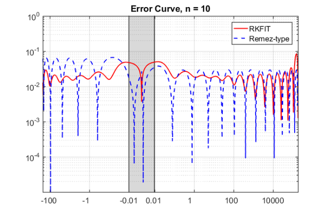
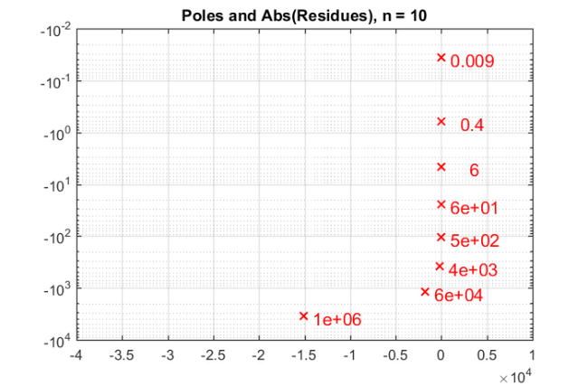
figure
semilogy(err_rkfit,'r-o'), hold on
semilogy(err_zolo,'b--')
bnd = exp(-pi*sqrt(1:m)); % *sqrt(2) in the exponent for [0,b2]
semilogy(20*bnd,'k:')
xlabel('degree n'), ylabel('relative 2-norm error')
legend('RKFIT (iter)','Remez-type','exp(-pi*sqrt(n))')
labels = num2str(iter_rkfit(:),'%d');
hdl = text((1:m)-.4,err_rkfit/4, labels,'horizontal','left','vertical','bottom');
set(hdl,'FontSize',13,'Color','r')
axis([0,m+1,1e-7,1]), grid on
title('Convergence for Indefinite Interval')

Conclusions

The error of the Remez-type approximant, as well as the RKFIT approximant, seems to reduce like $\exp(-\pi\sqrt{n})$ . This is plausible in view of the results by Newman and Vjacheslavov: they showed that the error of the best uniform rational approximant to $\sqrt{\lambda}$ on a semi-definite interval $[0,b_2]$ reduces like $\exp(-\pi\sqrt{2n})$ with the degree $n$ ; see Section 4 in [2]. Here we seem to lose a factor of $2$ because we are approximating on the union of two semi-definite intervals.

Other examples

The other examples in [1] can be reproduced with the following scripts:

Figure 1.2 - an infinite waveguide with two layers

Example 6.1 - constant coefficient and 1D indefinite Laplacian

Example 6.2 - constant coefficient and 2D indefinite Laplacian

Example 7.1 - truly variable-coefficient case with 2D indefinite Laplacian

References

[1] V. Druskin, S. Güttel, and L. Knizhnerman. Compressing variable-coefficient exterior Helmholtz problems via RKFIT, MIMS EPrint 2016.53 (http://eprints.ma.man.ac.uk/2511/), Manchester Institute for Mathematical Sciences, The University of Manchester, UK, 2016.

[2] P. P. Petrushev and V. A. Popov. Rational Approximation of Real Functions, Cambridge Univ. Press, Cambridge, 1987.