Compressing exterior Helmholtz problems: 3D layered waveguide

Stefan Güttel, October 2016Download PDF or m-file

Introduction
The code
Conclusions
Other examples
References

Introduction

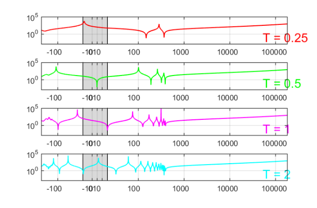
This script reproduces Example 7.1 in [1]. It computes RKFIT approximants for $f_h(A)\mathbf{b}$ , where $A$ is an indefinite matrix corresponding to the discretization of a 2D Laplacian on a square domain with Neumann boundary conditions; hence DCT2 can be used to diagonalize this matrix. The function $f_h$ to be approximated is a rather complicated DtN function due to the variability of the coefficient.

The code

n = 150; N = n^2;
h = 1/n; % grid step (now including boundary points for Neumann bcs)
k = 15;
L = gallery('tridiag',n); L(1,1) = 1; L(n,n) = 1;
L2 = kron(speye(n),L) + kron(L,speye(n));
eeL = 2-2*cos(pi*(0:n-1)/n).'; % evs of L
[ee1,ee2] = meshgrid(eeL);
eeL2 = (ee1(:)+ee2(:)); % evs of L2 ordered for DCT
% fL2v computes f(L2)*v using 2d DCT
fL2v = @(f,v) reshape(idct2(reshape(f(eeL2) .* ...
    reshape(dct2(reshape(v,n,n)),N,1),n,n)),N,1);
fL2V = @(f,V) util_colfun(@(v) fL2v(f,v),V);

% matrix A and matrix-vector product AV
A = 1/h^2*L2 - k^2*speye(N);
AV = @(V) fL2V(@(z) z/h^2-k^2,V);

% handles for rkfit
AB.solve = @(nu, mu, x) fL2v(@(z) 1./(nu*(z/h^2-k^2)-mu),x);
AB.multiply = @(rho, eta, x) fL2v(@(z) rho*(z/h^2-k^2)-eta,x);

% multipy with f(A)
fAV = @(f,V) fL2V(@(z) f(z/h^2-k^2),V);

% eigenvalues and spectral interval bounds
ee = sort(eeL2/h^2 - k^2).';           %ee = sort(eig(full(A))).';
a1 = min(ee);
b1 = max(ee(ee<0));
a2 = min(ee(ee>0));
b2 = max(ee);

bt = randn(N,1); bt = bt/norm(bt); % training vector
b  = randn(N,1); b = b/norm(b);    % testing vector

% Initialize RKFIT parameters
param = struct;
param.reduction = 0;
param.k = 1; % superdiagonal
param.tol = 0;
param.real = 0;

Thick = [ 0.25, 0.5 , 1 , 2  ];
Colors = { 'r','g','m','c' };
set(0,'RecursionLimit',700);

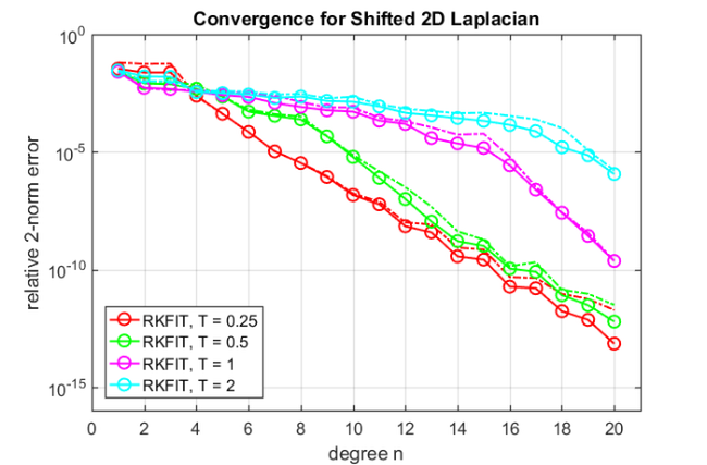
for j = 1:length(Thick), % loop over different layer thicknesses

    % Here is the definition of the variable coefficient function c.
    % Positive values of c "make A more definite" (e.g., if set to c=+k^2,
    % there is no shift in A at all). You can easily modify c(x).
    thick = Thick(j);
    v = [ 0 , 0 , 125*ones(1,round(thick/h)) , -400*ones(1,round(thick/h)) ];
    ex = util_dtnfun(h,v);

    % plot DtN function f_h
    figure(1), subplot(4,1,j)
    semilogy(NaN), hold on
    lint = util_log2lin([b1,a2],[a1,b1,a2,b2],.1);
    fill([lint(1:2),lint([2,1])], [1e-25,1e-25,1e15,1e15], ...
        .85*[1,1,1], 'LineStyle', '-')
    ylim([1e-3,1e5]), ax = [ -10.^(5:-1:1) , 0 , 10.^(1:5) ];
    linax = util_log2lin(ax,[a1,b1,a2,b2],.1);
    set(gca,'XTick',linax,'XTickLabel',ax)
    xlim([0,1]), grid on, set(gca,'layer','top')
    xx = sort([ -logspace(log10(-a1),log10(-b1),1000) , linspace(b1,a2,200) , ...
        logspace(log10(a2),log10(b2),1000) ]);
    xxt = util_log2lin(xx.',[a1,b1,a2,b2],.1).';
    semilogy(xxt,abs(ex(xx)),'r-','Color',Colors{j});
    hdl = text(.90,.1,['T = ' num2str(thick) ] );
    set(hdl,'FontSize',20,'Color',Colors{j})

    % define multiplication with DtN map
    %FV = @(V) fAV(ex,V); % very slow!
    fex = ex(eeL2/h^2 - k^2);
    fex2 = @(x) fex;
    FV = @(V) fAV(fex2,V); % faster!

    for m = 1:20, % loop over approximation degrees

        % run rkfit
        param.maxit = 10;
        xi = inf(1,m-1); % m-1 initial poles at infinity
        [xi,ratfun,misfit,out] = rkfit(FV,AB,bt,xi,param);
        if m==1, err_rkfitt = out.misfit_initial; iter_rkfit = 0;
        else
            [err_rkfitt(m),iter_rkfit(m)] = min(misfit);
            iter_rkfit(m) = find(misfit <= 1.01*min(misfit),1);
        end

        % recompute best ratfun and compute error for vector b
        param.maxit = iter_rkfit(m);
        xi = inf(1,m-1); % take m-1 initial poles at infinity
        [xi,ratfun,misfit,out] = rkfit(FV,AB,bt,xi,param);
        err_rkfit(m) = norm(FV(b) - fAV(ratfun,b))/norm(FV(b));
    end % for m

    figure(2), hd(j) = semilogy(err_rkfitt,'r-o','Color',Colors{j});
    hold on, semilogy(err_rkfit,'r-.','Color',Colors{j})

    if 0, % plot iteration numbers
        labels = num2str(iter_rkfit(:),'%d');
        hdl = text((1:m)-.4, err_rkfitt/10, labels, 'horizontal', ...
            'left', 'vertical', 'bottom');
        set(hdl,'FontSize',13,'Color',Colors{j})
    end
end % j

figure(2)
xlim([0,m+1]), ylim([1e-16,1])
xlabel('degree n'), ylabel('relative 2-norm error')
legend(hd, 'RKFIT, T = 0.25', 'RKFIT, T = 0.5', 'RKFIT, T = 1', ...
    'RKFIT, T = 2', 'Location', 'SouthWest')
grid on, title('Convergence for Shifted 2D Laplacian')

Conclusions

Given the many singularities of the DtN function $f_h$ in the spectral interval of $A$ , we observe a remarkably robust RKFIT convergence. As the layer thickness $T$ increases, the approximation accuracy deteriorates as expected, but even in the most extreme case RKFIT converges reliably. It is easy to modify this code to other operators $A$ , or other coefficient functions $c(x)$ .

Other examples

The other examples in [1] can be reproduced with the following scripts:

Figure 1.2 - an infinite waveguide with two layers

Example 6.1 - constant coefficient and 1D indefinite Laplacian

Example 6.2 - constant coefficient and 2D indefinite Laplacian

Example 6.3 - uniform approximation on indefinite interval

References

[1] V. Druskin, S. Güttel, and L. Knizhnerman. Compressing variable-coefficient exterior Helmholtz problems via RKFIT, MIMS EPrint 2016.53 (http://eprints.ma.man.ac.uk/2511/), Manchester Institute for Mathematical Sciences, The University of Manchester, UK, 2016.