Compressing exterior Helmholtz problems: 1D indefinite Laplacian
Stefan GüttelDownload PDF or m-file
Contents
Introduction
This script reproduces Example 6.1 in [2]. It computes RKFIT approximants for  , where
  is a symmetric indefinite matrix corresponding to the discretization of a 1D Laplacian and
 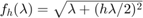 . The RKFIT approximants are compared to the uniform two-interval Zolotarev approximants in [1].
The code
N = 150;
h = 1/N; % grid step
k = 15;
L = gallery('tridiag',N); L(1,1) = 1; L(N,N) = 1;
A = 1/h^2*L - k^2*speye(N);
F = sqrtm(full(A) + (h*full(A)/2)^2);

bt = randn(N,1); bt = bt/norm(bt); % training vector
b = randn(N,1); b = b/norm(b);

ee = sort(eig(full(A))).';
a1 = min(ee);
b1 = max(ee(ee<0));
a2 = min(ee(ee>0));
b2 = max(ee);
Initialize RKFIT parameters.
param = struct;
param.reduction = 0;
param.k = 1; % superdiagonal
param.tol = 0;
param.real = 0;

for m = 1:25,

    % run rkfit with training vector
    param.maxit = 5;
    xi = inf*ones(1,m-1); % take m-1 initial poles
    [xi,ratfun,misfit,out] = rkfit(F,A,bt,xi,param);
    if m==1, err_rkfitt = out.misfit_initial; iter_rkfit = 0;
    else
        [err_rkfitt(m),iter_rkfit(m)] = min(misfit);
        iter_rkfit(m) = find(misfit <= 1.01*min(misfit),1);
    end

    % recompute best ratfun and compute error for vector b
    param.maxit = iter_rkfit(m);
    xi = inf*ones(1,m-1); % take m-1 initial poles
    [xi,ratfun,misfit,out] = rkfit(F,A,bt,xi,param);
    err_rkfit(m) = norm(F*b - ratfun(A,b))/norm(F*b);

    ex = @(x) sqrt(x + (h*x/2).^2);
    zolo = rkfun('sqrt2h',a1,b1,a2,b2,m,h);
    % check matrix-vector error
    err_zolo(m) = norm(F*b - zolo(A,b))/norm(F*b);

    if m == 10, % some plots for m = 10

        figure
        semilogy(NaN); hold on
        lint = util_log2lin([b1,a2],[a1,b1,a2,b2],.1);
        fill([lint(1:2),lint([2,1])], [1e-25,1e-25,1e15,1e15], ...
            .85*[1,1,1], 'LineStyle', '-')
        ylim([1e-10,10])
        ax = [ -10.^(5:-1:2) , 0 , 10.^(2:5) ];
        linax = util_log2lin(ax,[a1,b1,a2,b2],.1);
        %labels = num2str(ax(:),'%1.0G');
        set(gca,'XTick',linax,'XTickLabel',ax)
        xx = [ -logspace(log10(-a1),log10(-b1),1000) , linspace(b1,a2,200) , ...
            logspace(log10(a2),log10(b2),1000) ];
        xx = union(xx,ee);
        xxt = util_log2lin(xx,[a1,b1,a2,b2],.1);
        eet = util_log2lin(ee,[a1,b1,a2,b2],.1);
        hdl1 = semilogy(xxt,abs(ratfun(xx) - ex(xx)),'r-');
        semilogy(eet,abs(ratfun(ee) - ex(ee)),'r+')
        hdl2 = semilogy(xxt,abs(zolo(xx) - ex(xx)),'b--');
        legend([hdl1,hdl2],'RKFIT','Zolotarev ')
        xlim([0,1])
        title(['Error Curves, n = ' num2str(m) ])
        grid on
        set(gca,'layer','top')

        % plot residues
        figure
        [resid,xi] = residue(mp(ratfun),2);
        resid = double(resid); xi = double(xi);
        semilogy(xi,'rx')
        axis([-6.2e4,1.2e4,-6e3,-1e1]), hold on
        labels = num2str(abs(resid),'%0.1g');
        hdl = text(real(xi)+1e3, imag(xi)*1.1, labels);
        set(hdl,'Color','r','FontSize',16,'Rotation',0)
        set(hdl(end),'Rotation',0)
        title(['Poles and Abs(Residues), n = ' num2str(m)])
        grid on

        % plot grid steps
        figure
        [grid1,grid2,absterm,cnd,pf] = contfrac(mp(ratfun));
        grid1 = double(grid1); grid2 = double(grid2);
        loglog(grid1,'ro'), hold on
        loglog(grid2,'r*')
        legend('Primal','Dual','Location','SouthWest')
        title(['Grid Steps, n = ' num2str(m)]), grid on
        axis([2e-3,5e-1,-1,-1e-8])
    end
end % for m
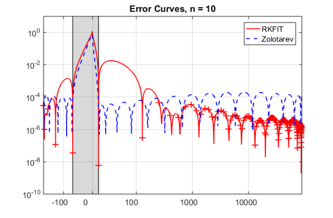
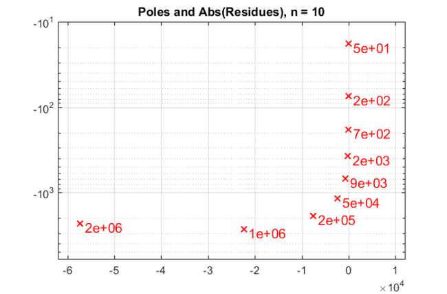
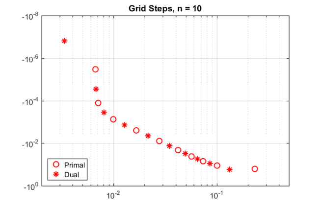
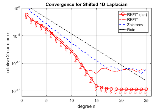
figure
semilogy(err_rkfitt,'r-o')
hold on
semilogy(err_rkfit,'r-.')
semilogy(err_zolo,'b--')
rate = exp(-2*pi^2/log((256*a1*b2/a2/b1)));
semilogy(10*rate.^(1:m),'k:')
ylim([1e-16,1])
xlim([0,m+1])
xlabel('degree n')
ylabel('relative 2-norm error')
legend('RKFIT (iter)','RKFIT','Zolotarev','Rate')
labels = num2str(iter_rkfit(:),'%d');
hdl = text((1:m)-.4,err_rkfitt/10,labels,'horizontal','left','vertical','bottom');
set(hdl,'FontSize',13,'Color','r'), grid on
title('Convergence for Shifted 1D Laplacian')
Conclusions
The main observation is that, due to spectral adaptation, the RKFIT approximants significantly outperform the uniform Zolotarev approximants and yield superlinear convergence in accuracy. Only a small number of RKFIT iterations is required to compute these approximants.
Other examples
The other examples in [2] can be reproduced with the following scripts:
Figure 1.2 - an infinite waveguide with two layers
Example 6.2 - constant coefficient and 2D indefinite Laplacian
Example 6.3 - uniform approximation on indefinite interval
Example 7.1 - truly variable-coefficient case with 2D indefinite Laplacian
References
[1] V. Druskin, S. Güttel, and L. Knizhnerman. Near-optimal perfectly matched layers for indefinite Helmholtz problems, SIAM Rev., 58(1):90--116, 2016.
[2] V. Druskin, S. Güttel, and L. Knizhnerman. Compressing variable-coefficient exterior Helmholtz problems via RKFIT, MIMS EPrint 2016.53 (http://eprints.ma.man.ac.uk/2511/), Manchester Institute for Mathematical Sciences, The University of Manchester, UK, 2016.