Compressing exterior Helmholtz problems: 2D indefinite Laplacian

Stefan Güttel, October 2016Download PDF or m-file

Introduction
The code
Conclusions
Other examples
References

Introduction

This script reproduces Example 6.2 in [2]. It computes RKFIT approximants for $f_h(A)\mathbf{b}$ , where $A$ is an indefinite matrix corresponding to the discretization of a 2D Laplacian on a square domain with Neumann boundary conditions; hence DCT2 can be used to diagonalize this matrix. The function to be approximated is 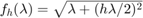$f_h(\lambda) = \sqrt{\lambda + (h\lambda/2)^2}$ . The RKFIT approximants are compared to the uniform two-interval Zolotarev approximants in [1].

The code

n = 150; N = n^2;
h = 1/n; % grid step (now including boundary points for Neumann bcs)
k = 15;
L = gallery('tridiag',n); L(1,1) = 1; L(n,n) = 1;
L2 = kron(speye(n),L) + kron(L,speye(n));
eeL = 2-2*cos(pi*(0:n-1)/n).'; % evs of L
[ee1,ee2] = meshgrid(eeL);
eeL2 = (ee1(:)+ee2(:)); % evs of L2 ordered for DCT
% fL2v computes f(L2)*v using 2d DCT
fL2v = @(f,v) reshape(idct2(reshape(f(eeL2) .* ...
    reshape(dct2(reshape(v,n,n)),N,1),n,n)),N,1);
fL2V = @(f,V) util_colfun(@(v) fL2v(f,v),V);

% matrix A and matrix-vector product AV
A = 1/h^2*L2 - k^2*speye(N);
AV = @(V) fL2V(@(z) z/h^2-k^2,V);

% handles for rkfit
AB.solve = @(nu, mu, x) fL2v(@(z) 1./(nu*(z/h^2-k^2)-mu),x);
AB.multiply = @(rho, eta, x) fL2v(@(z) rho*(z/h^2-k^2)-eta,x);

% multipy with f(A)
fAV = @(f,V) fL2V(@(z) f(z/h^2-k^2),V);

% multiply with analytic DtN map
ee = sort(eeL2/h^2 - k^2).';           %ee = sort(eig(full(A))).';
%F = sqrtm(full(A) + (h*full(A)/2)^2);
FV = @(V) fAV(@(z) sqrt(z+(h*z/2).^2),V);

bt = randn(N,1); bt = bt/norm(bt); % training vector
b  = randn(N,1); b = b/norm(b);

a1 = min(ee);
b1 = max(ee(ee<0));
a2 = min(ee(ee>0));
b2 = max(ee);

Initialize RKFIT parameters.

param = struct;
param.reduction = 0;
param.k = 1; % superdiagonal
param.tol = 0;
param.real = 0;

for m = 1:20, % in the paper [2] this is 25

    % run rkfit with training vector
    param.maxit = 10;
    xi = inf*ones(1,m-1); % take m-1 initial poles
    [xi,ratfun,misfit,out] = rkfit(FV,AB,bt,xi,param);
    if m==1, err_rkfitt = out.misfit_initial; iter_rkfit = 0;
    else
        [err_rkfitt(m),iter_rkfit(m)] = min(misfit);
        iter_rkfit(m) = find(misfit <= 1.01*min(misfit),1);
    end

    % recompute best ratfun and compute error for vector b
    param.maxit = iter_rkfit(m);
    xi = inf*ones(1,m-1); % take m-1 initial poles
    [xi,ratfun,misfit,out] = rkfit(FV,AB,bt,xi,param);
    err_rkfit(m) = norm(FV(b) - fAV(ratfun,b))/norm(FV(b));

    ex = @(x) sqrt(x + (h*x/2).^2);
    zolo = rkfun('sqrt2h',a1,b1,a2,b2,m,h);
    err_zolo(m) = norm(FV(b) - fAV(@(z) zolo(z),b))/norm(FV(b));

    if m == 10, % some plots for m = 10
        figure
        semilogy(NaN); hold on
        lint = util_log2lin([b1,a2],[a1,b1,a2,b2],.1);
        fill([lint(1:2),lint([2,1])], [1e-25,1e-25,1e15,1e15], ...
            .85*[1,1,1], 'LineStyle', '-')
        ylim([1e-8,10])
        ax = [ -10.^(5:-1:2) , 0 , 10.^(2:5) ];
        linax = util_log2lin(ax,[a1,b1,a2,b2],.1);
        %labels = num2str(ax(:),'%1.0G');
        set(gca,'XTick',linax,'XTickLabel',ax)

        xx = [ -logspace(log10(-a1),log10(-b1),1000) , linspace(b1,a2,200) , ...
            logspace(log10(a2),log10(b2),1000) ];
        xx = union(xx,ee);
        xxt = util_log2lin(xx,[a1,b1,a2,b2],.1);
        eet = util_log2lin(ee,[a1,b1,a2,b2],.1);
        hdl1 = semilogy(xxt,abs(ratfun(xx) - ex(xx)),'r-');
        semilogy(eet,abs(ratfun(ee) - ex(ee)),'r+')
        hdl2 = semilogy(xxt,abs(zolo(xx) - ex(xx)),'b--');
        legend([hdl1,hdl2],'RKFIT','Zolotarev ')
        xlim([0,1])
        title(['Error Curves, n = ' num2str(m) ])
        grid on
        set(gca,'layer','top')

        % plot residues
        figure
        [resid,xi] = residue(mp(ratfun),2);
        resid = double(resid); xi = double(xi);
        semilogy(xi,'rx')
        axis([-6.2e4,1.2e4,-5e3,-5]), hold on
        labels = num2str(abs(resid),'%0.1g');
        hdl = text(real(xi)+1e3, imag(xi)*1.1, labels);
        set(hdl,'Color','r','FontSize',16,'Rotation',0)
        set(hdl(end),'Rotation',0)
        title(['Poles and Abs(Residues), n = ' num2str(m)])
        grid on

        % plot grid steps
        figure
        [grid1,grid2,absterm,cnd,pf,Q] = contfrac(mp(ratfun));
        grid1 = double(grid1); grid2 = double(grid2);
        loglog(grid1,'ro'), hold on
        loglog(grid2,'r*')
        legend('Primal','Dual','Location','SouthWest')
        title(['Grid Steps, n = ' num2str(m)])
        grid on, axis([2e-3,5e-1,-1,-1e-8])

        % plot solution slices
        figure
        U = out.V*double(Q); % first col = F*b, then U0,U1,etc.
        U(:,2) = b; % get rid of tiny imaginary parts if b is real
        Vol = []; % build volume object
        for j = 2:size(U,2),
            Vol(:,j-1,:) = reshape(U(:,j),n,n);
        end
        neps = min(min(min(abs(Vol))))/1;
        Vol(:,j,:) = zeros(n,n)+neps;
        [x,y,z] = meshgrid(0:1:j-1,linspace(0,1,n),linspace(0,1,n));
        xslice = 0:1:j-1; yslice = []; zslice = [];
        hdl = slice(x,y,z,log10(abs(Vol)),xslice,yslice,zslice);
        set(hdl,'FaceAlpha',1,'LineStyle','none')
        set(gca,'Color',[0 0 0]), colorbar
        set(gca,'CLim',[-5,-2]), view(-7,16)
        set(gca,'XTick',0:100,'YTick',0:.5:1,'ZTick',0:.5:1)
        title(['Amplitude, n = ' num2str(m)])

        figure
        Ang = angle(Vol); Ang(Ang<0) = 2*pi+Ang(Ang<0);
        hdl = slice(x,y,z,Ang,xslice,yslice,zslice);
        set(hdl,'FaceAlpha',1,'LineStyle','none')
        set(gca,'Color',[0 0 0]), set(gca,'CLim',[0,2*pi])
        colorbar, view(-7,16)
        set(gca,'XTick',0:100,'YTick',0:.5:1,'ZTick',0:.5:1)
        title(['Phase, n = ' num2str(m)])
    end
end % for m

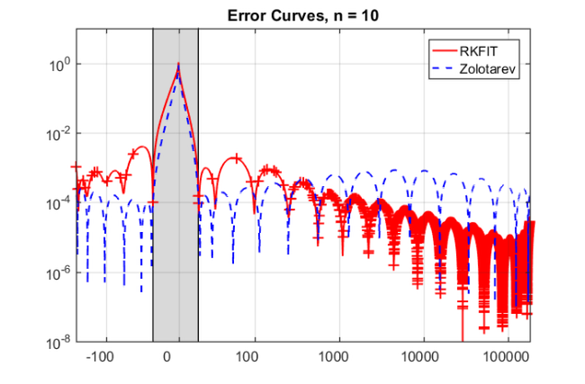
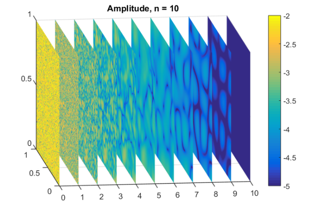
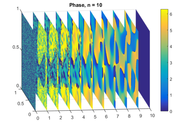
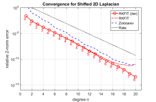
figure
semilogy(err_rkfitt,'r-o'), hold on
semilogy(err_rkfit,'r-.')
semilogy(err_zolo,'b--')
rate = exp(-2*pi^2/log((256*a1*b2/a2/b1)));
semilogy(10*rate.^(1:m),'k:')
ylim([1e-16,1]), xlim([0,m+1])
xlabel('degree n')
ylabel('relative 2-norm error')
legend('RKFIT (iter)','RKFIT','Zolotarev','Rate')
labels = num2str(iter_rkfit(:),'%d');
hdl = text((1:m)-.4,err_rkfitt/10,labels,'horizontal','left','vertical','bottom');
set(hdl,'FontSize',13,'Color','r'), grid on
title('Convergence for Shifted 2D Laplacian')

Conclusions

The main observation is that for this 2D problem the RKFIT approximants perform very similar to the uniform Zolotarev approximants. Compared to the 1D Laplacian example, no significant superlinear convergence effects are observed. Still the number of required RKFIT iterations is very small.

Other examples

The other examples in [2] can be reproduced with the following scripts:

Figure 1.2 - an infinite waveguide with two layers

Example 6.1 - constant coefficient and 1D indefinite Laplacian

Example 6.3 - uniform approximation on indefinite interval

Example 7.1 - truly variable-coefficient case with 2D indefinite Laplacian

References

[1] V. Druskin, S. Güttel, and L. Knizhnerman. Near-optimal perfectly matched layers for indefinite Helmholtz problems, SIAM Rev., 58(1):90--116, 2016.

[2] V. Druskin, S. Güttel, and L. Knizhnerman. Compressing variable-coefficient exterior Helmholtz problems via RKFIT, MIMS EPrint 2016.53 (http://eprints.ma.man.ac.uk/2511/), Manchester Institute for Mathematical Sciences, The University of Manchester, UK, 2016.