Model order reduction example
Mario Berljafa and Stefan Güttel, May 2016Download PDF or m-file
Contents
Introduction
This script reproduces the numerical example from [2, Sec. 5.2], which relates to the INLET problem from the Oberwolfach Model Reduction Benchmark Collection [1], an active control model of a supersonic engine inlet; see also [3]. We demonstrate our near-optimal continuation strategy for approximating the transfer function of a dynamical system. In this experiment the number of parallel processors varies.
MATLAB code
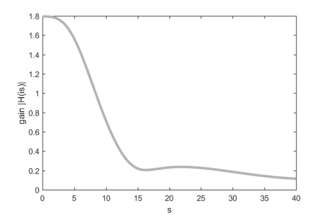
Let us load the data and plot the exact transfer function.
if exist('Inlet.A') ~= 2 || exist('Inlet.B') ~= 2 || ...
   exist('Inlet.C') ~= 2 || exist('Inlet.E') ~= 2 || ...
   exist('mmread') ~= 2
   disp(['The required matrices for this problem can be '  ...
         'downloaded from https://portal.uni-freiburg.de/' ...
         'imteksimulation/downloads/benchmark/38866']);
   return
end

N = 11730;
A = mmread('oberwolfach_inlet/Inlet.A');
B = mmread('oberwolfach_inlet/Inlet.B'); B = B(:,1);
C = mmread('oberwolfach_inlet/Inlet.C');
E = mmread('oberwolfach_inlet/Inlet.E');
f = @(s) full(C*((s*E - A)\B));

f0 = 40;
s = linspace(0, f0, 12 + 11*8);
for j = 1:length(s), fs(j) = f(1i*s(j)); end

figure(1)
plot(s, abs(fs), 'k-', 'Color', [0.7,0.7,0.7], 'LineWidth', 4)
xlabel('s'), ylabel('gain |H(is)|'), hold on
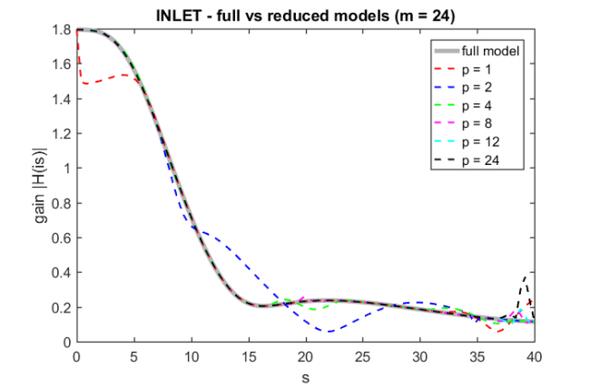
Now we use the rat_krylov function simulating a varying number p of parallel processors to compute reduced order models.
P   = [1, 2, 4, 8, 12, 24];
col = {'r', 'b', 'g', 'm','c', 'k'};

ucf = @(AB, nu, mu, x, param) ...
      util_continuation_fom(AB, nu, mu, x, param);

param.continuation       = 'near-optimal';
param.continuation_m     = 5;
param.continuation_root  = inf;
param.continuation_solve = ucf;
param.orth               = 'CGS';
param.reorth             = 0;
param.waitbar            = 1;

for indp = 1:length(P)
  p = P(indp);
  if p > 1
    xi = 1i*repmat(linspace(0, f0, p), 1, 24/p);
  else
    xi = 1i*f0/2*ones(1, 24);
  end

  param.p = p;

  [V, K, H, out] = rat_krylov(A, E, full(A\B), xi, param);

  fprintf('p = %d\n', p)

  % Numerical quantities (cf. [1, Figure 5.2]).
  EV = E*V; AV = A*V; S = A\EV; S = S-V*(V\S); ss = svd(S);
  R = out.R;
  D = fminsearch(@(x) cond(R*diag(x)), ones(size(R, 2), 1), ...
                 struct('Display','off'));
  nrm = norm(V'*V - eye(size(V,2)));

  fprintf('   Cond number (scaled): %.3e\n', cond(R*diag(D)))
  fprintf('   Orthogonality check:  %.3e\n', nrm)
  fprintf('   sigma_2/sigma_1:      %.3e\n\n', ss(2)/ss(1))

  % Evaluate and plot reduced transfer function.
  Em = V'*E*V; Am = V'*A*V; Bm = V'*B; Cm = C*V;
  for j = 1:length(s)
    fsm(j) = (Cm*((1i*s(j)*Em - Am)\Bm));
  end
  plot(s, abs(fsm), '--', 'Color', col{indp})
end

title('INLET - full vs reduced models (m = 24)')
legend('full model', ...
       'p = 1', 'p = 2',  'p = 4', ...
       'p = 8', 'p = 12', 'p = 24')
p = 1
   Cond number (scaled): 1.811e+03
   Orthogonality check:  1.660e-12
   sigma_2/sigma_1:      1.027e-13

p = 2
   Cond number (scaled): 1.097e+04
   Orthogonality check:  2.198e-11
   sigma_2/sigma_1:      2.758e-11

p = 4
   Cond number (scaled): 5.496e+02
   Orthogonality check:  7.550e-13
   sigma_2/sigma_1:      2.901e-13

p = 8
   Cond number (scaled): 6.083e+03
   Orthogonality check:  1.566e-11
   sigma_2/sigma_1:      2.273e-12

p = 12
   Cond number (scaled): 1.192e+04
   Orthogonality check:  1.393e-09
   sigma_2/sigma_1:      9.424e-12

p = 24
   Cond number (scaled): 4.835e+04
   Orthogonality check:  1.092e-01
   sigma_2/sigma_1:      6.682e-11
Links to other examples
Here is a list of other numerical illustrations of parallelization strategies:
Overview of the parallelization options
Numerical illustration from [2, Sec. 3.4]
TEM example from [2, Sec. 5.1]
Waveguide example from [2, Sec. 5.3]
References
[1] Oberwolfach Model Reduction Benchmark Collection, 2003. http://www.imtek.de/simulation/benchmark.
[2] M. Berljafa and S. Güttel. Parallelization of the rational Arnoldi algorithm, SIAM J. Sci. Comput., 39(5):S197--S221, 2017.
[3] G. Lassaux and K. Willcox. Model reduction for active control design using multiple-point Arnoldi methods, AIAA Paper, 616:1--11, 2003.