Waveguide example

Mario Berljafa and Stefan Güttel, May 2016Download PDF or m-file

Introduction
MATLAB code
Parallel variants
Links to other examples
References

Introduction

This script reproduces the waveguide example from [1, Sec. 5.3], where a detailed discussion can be found.

MATLAB code

We first load the data, and a few of the "exact" eigenvalues of $A$ (precomputed with MATLAB's eigs).

if exist('waveguide3D.mat') ~= 2
  disp('File waveguide3D.mat not found. Downloadable from:')
  disp(['http://www.cise.ufl.edu/research/sparse/' ...
	'matrices/FEMLAB/waveguide3D.html'])
  return
end

N = 21036;
load waveguide3D
A = Problem.A;

try, load waveguide3D_ee; catch, ee = []; end

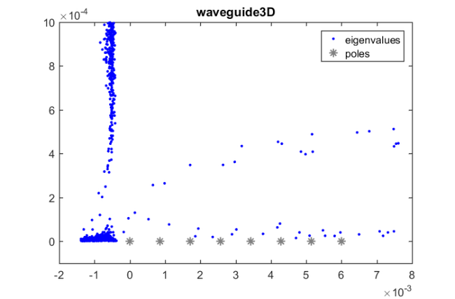
Here's some further initialisation and a plot of the eigenvalues and poles we want to use in the rational Krlov method.

b = ones(N, 1);
p = 8; rep = 8;
shift = 3e-3; % harmonic target
Xi = linspace(0, 6e-3, p);
Xi = Xi([1, 5, 3, 6, 2, 7, 4, 8]);
xi = repmat(Xi, 1, rep);
m  = length(xi);

figure(1)
plot(ee, 'b.'), hold on
plot(real(Xi), imag(Xi), 'k*', 'Color', [0.5, 0.5, 0.5])
legend('eigenvalues', 'poles', 'Location', 'NorthEast')
title('waveguide3D')
axis([-2e-3, 8e-3, -1e-4, 1e-3])

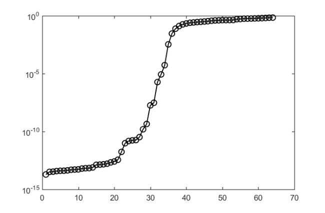
disp(['Running Ruhe sequential strategy'])

param = struct('continuation', 'ruhe', ...
               'orth',         'MGS',  ...
               'reorth',       1,      ...
               'waitbar',      1);

[V, K, H, out] = rat_krylov(A, b, xi, param);

AV = A*V; S = AV; S = S-V*(V\S); s = svd(S); R = out.R;
D = fminsearch(@(x) cond(R*diag(x)), ones(size(R, 2), 1), ...
               struct('Display','off'));
nrm = norm(V'*V - eye(size(V,2)));

fprintf('   Cond number (scaled): %.3e\n', cond(R*diag(D)))
fprintf('   Orthogonality check:  %.3e\n', nrm)
fprintf('   sigma_2/sigma_1:      %.3e\n\n', s(2)/s(1))

H = H - shift*K; [X,ritz] = eig(K'*H,K'*K);
ritz = diag(ritz) + shift; X = V*K*X;

[Res,ind] = sort(sqrt(sum(abs(A*X - X*diag(ritz)).^2))./ ...
                 (sqrt(sum(abs(A*X).^2)) + ...
                  sqrt(sum(abs(X*diag(ritz)).^2))));

figure(2), semilogy(Res,'k-o'), hold on

Running Ruhe sequential strategy
   Cond number (scaled): 1.578e+03
   Orthogonality check:  7.330e-15
   sigma_2/sigma_1:      1.868e-13

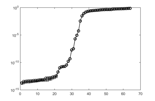
disp(['Running optimal sequential strategy'])

param.continuation = 'near-optimal';

[V, K, H, out] = rat_krylov(A, b, xi, param);

AV = A*V; S = AV; S = S-V*(V\S); s = svd(S); R = out.R;
D = fminsearch(@(x) cond(R*diag(x)), ones(size(R, 2), 1), ...
               struct('Display','off'));
nrm = norm(V'*V - eye(size(V,2)));

fprintf('   Cond number (scaled): %.3e\n', cond(R*diag(D)))
fprintf('   Orthogonality check:  %.3e\n', nrm)
fprintf('   sigma_2/sigma_1:      %.3e\n\n', s(2)/s(1))


H = H - shift*K; [X,ritz] = eig(K'*H,K'*K);
ritz = diag(ritz) + shift; X = V*K*X;

[Res,ind] = sort(sqrt(sum(abs(A*X - X*diag(ritz)).^2))./ ...
                 (sqrt(sum(abs(A*X).^2)) + ...
                  sqrt(sum(abs(X*diag(ritz)).^2))));

figure(2), semilogy(Res,'k-s'), hold on

Running optimal sequential strategy
   Cond number (scaled): 1.070e+00
   Orthogonality check:  7.329e-15
   sigma_2/sigma_1:      8.870e-15

Parallel variants

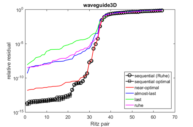
Here we compare four different continuation strategies for the parallel rational Arnoldi simulating $p=8$ cores.

strat = {'near-optimal', 'almost-last', 'last', 'ruhe'};
col   = {'r', 'b', 'g', 'm'};
ucf   = @(AB, nu, mu, x, param) ...
        util_continuation_fom(AB, nu, mu, x, param);
p = 8;

param.p = p;
param.continuation_m    = 5;
param.continuation_root = inf;

for s = 1:length(strat)
  disp(['Running strategy ' strat{s}])

  param.continuation = strat{s};

  [V, K, H, out] = rat_krylov(A, b, xi, param);

  AV = A*V; S = AV; S = S-V*(V\S); ss = svd(S); R = out.R;
  D = fminsearch(@(x) cond(R*diag(x)), ones(size(R, 2), 1), ...
                 struct('Display','off'));
  nrm = norm(V'*V - eye(size(V,2)));

  fprintf('   Cond number (scaled): %.3e\n', cond(R*diag(D)))
  fprintf('   Orthogonality check:  %.3e\n', nrm)
  fprintf('   sigma_2/sigma_1:      %.3e\n\n', ss(2)/ss(1))

  H = H - shift*K; [X,ritz] = eig(K'*H,K'*K);
  ritz = diag(ritz) + shift; X = V*K*X;

  Res = sort(sqrt(sum(abs(A*X - X*diag(ritz)).^2))./ ...
             (sqrt(sum(abs(A*X).^2)) + ...
              sqrt(sum(abs(X*diag(ritz)).^2))));

  ritz = ritz(ind);
  if s==1
    ritz = ritz(Res < 1e-8);
    figure(1), hold on
    plot(real(ritz), imag(ritz), 'o', 'Color', col{s})
  end

  figure(2), semilogy(Res, 'Color', col{s}), hold on
end

figure(1), title('waveguide3D')
legend('eigenvalues', 'poles', 'Ritz vals (near optimal)')

figure(2), title('waveguide3D')
xlabel('Ritz pair'), ylabel('relative residual')

legend('sequential (Ruhe)', 'sequential optimal', ...
       'near-optimal', 'almost-last', 'last',     ...
       'ruhe', 'Location', 'SouthEast')

Running strategy near-optimal
   Cond number (scaled): 2.103e+04
   Orthogonality check:  7.330e-15
   sigma_2/sigma_1:      7.514e-12

Running strategy almost-last
   Cond number (scaled): 5.619e+15
   Orthogonality check:  7.331e-15
   sigma_2/sigma_1:      9.587e-02

Running strategy last
   Cond number (scaled): 6.577e+08
   Orthogonality check:  7.330e-15
   sigma_2/sigma_1:      2.977e-08

Running strategy ruhe
   Cond number (scaled): 4.656e+08
   Orthogonality check:  7.330e-15
   sigma_2/sigma_1:      1.098e-08

References

[1] M. Berljafa and S. Güttel. Parallelization of the rational Arnoldi algorithm, SIAM J. Sci. Comput., 39(5):S197--S221, 2017.
[2] T. A. Davis and Y. Hu. The University of Florida Sparse Matrix Collection, ACM Trans. Math. Software, 38:1--25, 2011.