Transient electromagnetics example

Mario Berljafa and Stefan Güttel, May 2016Download PDF or m-file

Introduction
Rational Arnoldi approximation
Sequential reference solution
Parallel Arnoldi variants
Links to other examples
References

Introduction

This example relates to the modeling of a transient electromagnetic field in a geophysical application [2]. We consider here the first test problem in [2, Sec 5.1], the discretization of a layered half space using Nedelec elements of order $1$ . We are given a symmetric positive semidefinite matrix $A$ and a symmetric positive definite matrix $B$ , both of order $N=27623$ , and the task is to solve an initial value problem

$B \mathbf{e}'(t) + A \mathbf{e}(t) = \mathbf{0}, \quad \mathbf{e}(0) = \mathbf{b},$

for the electric field $\mathbf{e}(t)$ . The time parameters of interest are $t\in T = [10^{-6},10^{-3}]$ .

First let us load the matrices $A$ and $B$ , and the initial vector $\mathbf{b}$ :

if exist('tem.mat') ~= 2
  disp('File tem.mat not found. Can be downloaded from:')
  disp('http://guettel.com/tem/TEM27623.mat') % TEM152078.mat
  return
end

load tem
A = Problem.C; B = Problem.M; b = B\Problem.q;
N = size(A,1);

Rational Arnoldi approximation

The approach suggested in [2] is to build a $B$ -orthonormal rational Krylov basis $V_{m+1}$ of $\mathcal{Q}_{m+1}(B^{-1}A,\mathbf{b},q_m)$ , where $B^{-1}A$ is never formed explicitly, and to extract Arnoldi approximants

$\mathbf{f}_m(t) = \|\mathbf{b}\|_B V_{m+1} \exp(-t A_{m+1})\mathbf{e}_1, \quad A_{m+1} = V_{m+1}^T A V_{m+1}$

for all desired time parameters $t\in T$ . Here $\|\mathbf{b} \|_B = (\mathbf{b}^T B\mathbf{b})^{1/2}$ . Following [2, Table 1] we use $p=4$ mutually distinct poles each repeated cyclically $9$ times, resulting in a rational Krylov space of order $m=36$ .

p = 4; rep = 9;
Xi = [-2.76e+04,-4.08e+04,-2.45e+06,-6.51e+06];

Sequential reference solution

The problem is large enough so that using MATLAB's expm is impractical for obtaining an accurate reference solution. We therefore run the Arnoldi method with the above poles for a few more cycles to obtain a high-order rational Arnoldi decomposition.

xi = repmat(Xi, 1, rep+9);
ip = @(x,y) y'*B*x;
b = b/sqrt(ip(b, b));

param =  struct('continuation',  'ruhe', ...
                'orth',          'MGS',  ...
                'reorth',        1,      ...
                'waitbar',       1,      ...
                'inner_product', ip);

[V, K, H, out] = rat_krylov(A, B, b, xi, param);

We now use the basis V to extract the high-order Arnoldi approximants, which we consider as the "exact" reference solution:

Am = V'*A*V;
t = logspace(-6, -3, 31);
for j = 1:length(t)
  exact(:, j) = V*(expm(-t(j)*Am)*eye(size(Am, 1), 1));
end

Parallel Arnoldi variants

Since version 2.4 of the RKToolbox, the rat_krylov function can simulate the parallel construction of a rational Krylov basis. This is done by imposing various nonzero patterns in the so-called "continuation matrix" $T$ [1]. Simply speaking, the $j$ -th column of this matrix contains the coefficients of the linear combination of $j$ rational Krylov basis vectors which have been used to compute the next $(j+1)$ -th basis vector. It is therefore an upper triangular matrix.

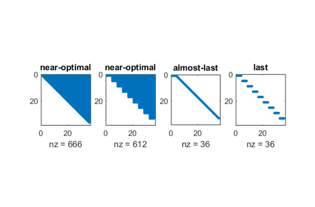
The following experiment tests and compares three different continuation strategies, including the "near-optimal" strategy proposed in [1]. This strategy is tested for both $p=1$ (sequential case) and $p=4$ . The other strategies almost-last and last are tested for $p=4$ . The predicting method is FOM(5), i.e., five iterations of the full orthogonalisaton method are used to predict the next Krylov basis vectors before actually computing them. The displayed quantities are indicators for the accuracy of the computed rational Arnoldi decomposition, and they are explained in details in [1]. The numbers should be comparable to this in Table 5.1 in [1]. Generally, smaller numbers are better. We also show the sparsity patterns of the various continuation matrices $T$ .

xi = repmat(Xi, 1, rep);
m  = length(xi);
strat = {'near-optimal', 'near-optimal', 'almost-last', 'last'};
ucf   = @(AB, nu, mu, x, param) ...
        util_continuation_fom(AB, nu, mu, x, param);

param.orth   = 'CGS';
param.reorth = 0;
param.continuation_m     = 5;
param.continuation_root  = inf;
param.continuation_solve = ucf;

for s = 1:length(strat)
  if s == 1
    p = 1; disp(['Sequential strategy ' strat{s}])
  else
    p = 4; disp(['Parallel strategy '   strat{s}])
  end

  param.p = p;
  param.continuation = strat{s};

  [V, K, H, out] = rat_krylov(A, B, b, xi, param);

  % Continuation matrix.
  figure(1), subplot(1, 4, s)
  spy(out.T), axis ij, title(strat{s})

  % Numerical quantities (cf. [1, Table 5.1]).
  BV = B*V; AV = A*V; S = B\AV; S = S-V*(V\S); ss = svd(S);
  R = out.R;
  D = fminsearch(@(x) cond(R*diag(x)), ones(size(R, 2), 1), ...
                 struct('Display','off'));
  nrm = norm(ip(V,V) - eye(size(V,2)));

  fprintf('   Cond number (scaled): %.3e\n', cond(R*diag(D)))
  fprintf('   Orthogonality check:  %.3e\n', nrm)
  fprintf('   sigma_2/sigma_1:      %.3e\n\n', ss(2)/ss(1))

  % Arnoldi approximations.
  Am = V'*A*V; t = logspace(-6, -3, 31);
  for j = 1:length(t)
    appr = V*(expm(-t(j)*Am)*eye(size(Am, 1), 1));
    d    = appr - exact(:,j);
    err(j,s) = sqrt(ip(d,d));
  end
end

Sequential strategy near-optimal
   Cond number (scaled): 7.531e+00
   Orthogonality check:  1.019e-14
   sigma_2/sigma_1:      3.843e-15

Parallel strategy near-optimal
   Cond number (scaled): 9.122e+02
   Orthogonality check:  1.306e-05
   sigma_2/sigma_1:      2.937e-14

Parallel strategy almost-last
   Cond number (scaled): 2.544e+18
   Orthogonality check:  1.596e+01
   sigma_2/sigma_1:      5.580e-07

Parallel strategy last
   Cond number (scaled): 1.289e+06
   Orthogonality check:  3.552e-01
   sigma_2/sigma_1:      2.663e-14

Finally, we show the absolute errors of the Arnoldi approximants depending on the time paramter $t$ . By construction in [2], these errors are guaranteed to satisfy $\|\mathbf{e}(t)-\mathbf{f}_m(t)\|_B \leq 6.74\times 10^{-8}$ for all $t\in T$ , independent of the spectral interval of $(A,B)$ :

figure(2), loglog(t, err), legend(strat)
title('Arnoldi approximants to exp(-tA)b')
xlabel('time t'), ylabel('M-norm error')
axis([1e-6, 1e-3, 1e-12, 1e-4])

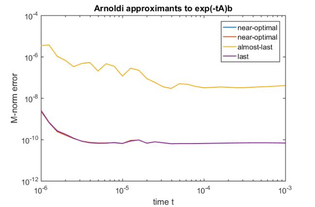
We clearly see that both the strategies last and almost-last suffer from numerical instability, whereas the near-optimal strategy works well both in the sequential and parallel case.

Links to other examples

Here is a list of other numerical illustrations of parallelization strategies:

Overview of the parallelization options

Numerical illustration from [1, Sec. 3.4]

Inlet example from [1, Sec. 5.2]

Waveguide example from [1, Sec. 5.3]

References

[1] M. Berljafa and S. Güttel. Parallelization of the rational Arnoldi algorithm, SIAM J. Sci. Comput., 39(5):S197--S221, 2017.

[2] R.-U. Börner, O. G. Ernst, and S. Güttel. Three-dimensional transient electromagnetic modeling using rational Krylov methods, Geophys. J. Int., 202(3):2025--2043, 2015.

[3] A. Ruhe. Rational Krylov: A practical algorithm for large sparse nonsymmetric matrix pencils, SIAM J. Sci. Comput., 19(5):1535--1551, 1998.