Near-optimal continuation pairs

Mario Berljafa and Stefan Güttel, May 2016Download PDF or m-file

Contents

Introduction

The MATLAB code provided here reproduces the numerical example from [2, Sec. 3.4]. This example demonstrates the effectiveness of the near-optimal strategy for selecting continuation pairs $(\eta_j/\rho_j, \mathbf{t}_j)$ used for the expansion of a rational Krylov space during the execution of the rational Arnoldi algorithm; see [2, Alg. 2.1] and [2, Sec. 2], where the notion of continuation pairs is introduced. In [2, Sec. 2-3] we propose and analyze a framework for selecting these continuation pairs in such a way as to minimize the growth of the condition number of the rational Krylov basis undergoing the Gram--Schmidt process in order to avoid numerical stability problems. The motivation for this work is to provide a robust parallel rational Arnoldi algorithm where numerical instability problems have been reported. For more details we refer to [2] and the references therein.

MATLAB code

In the remainder we provide and briefly comment on the MATLAB code. A detailed discussion of the example itself is provided in [2, Sec. 3.4].

We first setup the problem, similar to the one from [1, Sec. 5.3].

N = 1000; n = 300; m = 16;

% Surrogate problem to get the poles.
A = -5*gallery('grcar', n, 3);
b = ones(n, 1);
xi = rkfit(expm(full(A)), A, b, inf(1, m));

% Actual problem.
A = -5*gallery('grcar', N, 3);
b = ones(N, 1);

For the near-optimal continuation strategy we use FOM(2) and FOM(3).

ucf = @(AB, nu, mu, x, param) ...
      util_continuation_fom(AB, nu, mu, x, param);

param = struct('continuation', 'near-optimal', ...
               'continuation_solve',  ucf,     ...
               'continuation_bounds', true,    ...
               'orth',  'MGS',                 ...
               'reorth', 1);

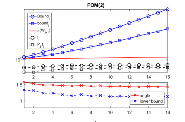
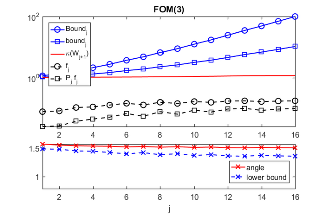
In the remainder we run the rational Arnoldi algorithm using rat_krylov first with FOM(2), and then with FOM(3) for the prediction of near-optimal continuation pairs.

for cntm = 2:3
  % Use FOM(cntm) to predict near-optimal continuation pairs.
  param.continuation_m = cntm;

  [V, K, H, out] = rat_krylov(A, b, xi, param);

  % This holds the norms of \widehat f_{j+1}.
  Delta = out.Fhat;

  % The following correspond to [2, eq. (3.20)].
  delta_u = 1 + 2*out.fhat + out.Fhat.^2;
  delta_l = 1 - 2*out.fhat;

  cond_number = @(X) arrayfun(@(j)cond(X(:, 1:j+1)), ...
                              1:size(X, 2)-1);

  % Bound from [2, Thm. 3.6].
  Bound = cumprod((1+Delta)./(1-Delta));
  % Analogous bound based on [2, eq. (3.20)].
  bound = sqrt(cumprod(delta_u./delta_l));

  figure(cntm-1)
  subplot(3, 1, 1:2)
  semilogy(Bound, 'bo-'), hold on
  semilogy(bound, 'bs-')
  semilogy(cond_number(out.W), 'r-')
  semilogy(out.Fhat, 'ko--')
  semilogy(out.fhat, 'ks--')

  legend('Bound_j', 'bound_j', '\kappa(W_{j+1})', ...
         'f_j', 'P_j f_j', 'location', 'NorthWest')

  xmin = 1;
  xmax = m;
  ymin = min([1, min(out.fhat)]);
  ymax = max(Bound);

  axis([xmin xmax ymin ymax])
  title(['FOM(' num2str(cntm) ')'])

  W = out.W;
  for j = 1:m
    num = norm(W(:, j+1)-V(:, 1:j)*(V(:, 1:j)'*W(:, j+1)));
    dnm = norm(V(:, 1:j)*(V(:, 1:j)'*W(:, j+1)));
    % Angle between w_{j+1} and range(V_j).
    angl(j) = atan(num/dnm);
    % Corresponding lower bound given by [2, Cor. 3.4].
    angl_bound(j) = atan(1/out.Fhat(j)-1);
  end

  subplot(3, 1, 3)
  plot(angl, 'rx-'), hold all
  plot(angl_bound, 'bx--')
  axis([xmin xmax pi/4 pi/2])
  legend('angle', 'lower bound', 'location', 'SouthEast')
  xlabel('j')
end

Links to other examples

Here is a list of other numerical illustrations of parallelization strategies:

Overview of the parallelization options

TEM example from [1, Sec. 5.1]

Inlet example from [1, Sec. 5.2]

Waveguide example from [1, Sec. 5.3]

References

[1] M. Berljafa and S. Güttel. Generalized rational Krylov decompositions with an application to rational approximation, SIAM J. Matrix Anal. Appl., 36(2):894--916, 2015.

[2] M. Berljafa and S. Güttel. Parallelization of the rational Arnoldi algorithm, SIAM J. Sci. Comput., 39(5):S197--S221, 2017.

Published with MATLAB® R2016a